|
김관석
|
2024-04-04 09:01:37, 조회수 : 103 |
- Download #1 : Wa_Fig_3cs.jpg (433.4 KB), Download : 3

3.4 Wave packets and dispersion
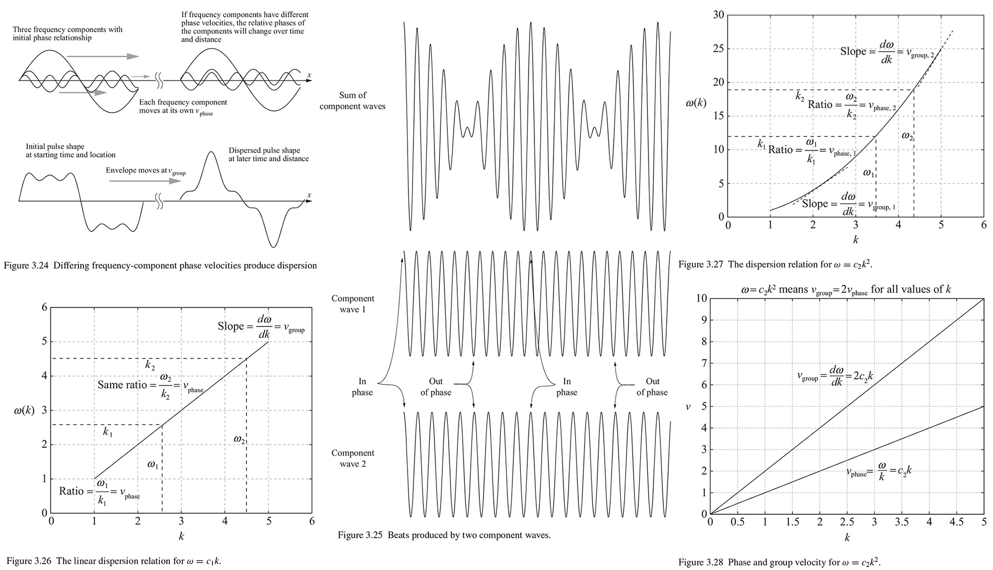
Consider what would happen if the frequency components that make up the waveform (called a "wave packet" if it's localized in time and space) had different speeds. We can see an example of that in Fig. 3.24.. Three frequency components have the right amplitude and frequency to add up to a square(ish) pulse at some initial location and time. But at a different location the relative phase between the component waves will be different. We can see the result of that change in relative phase in the bottom-right portion of the Fig. 3.24.: The shape of the resultant waveform changes over distance.
This effect is called "dispersion". And when dispersion is present, the speed of each individual frequency component is called the phase velocity or phase speeds of the component, and the speed of the wave packet's envelope is called the "group velocity" or group speed.(4) In order to understand the group velocity of a wave packet, look at an example shown in Fig. 3.25. Here the two component waves start off in phase and produce a large resultant wave. When the two component waves have slightly different frequencies and the amplitude of the resultant waveform varies as it does in Fig. 3.25, and the waveform is said to be "modulated", and this particular type of modulation is called "beats". The modulation envelope shown here provides a convenient way to determine the group velocity of a wave packet. To see how that works, write the phase of them as 𝜙 = 𝑘𝑥 - 𝜔𝑡,
𝜙1 = 𝑘1𝑥 - 𝜔1𝑡, 𝜙2 = 𝑘2𝑥 - 𝜔2𝑡.
This means that the phase difference between the wave is
𝛥𝜙 = 𝜙2 - 𝜙1 = (𝑘2𝑥 - 𝜔2𝑡) - (𝑘1𝑥 - 𝜔1𝑡) = (𝑘2 - 𝑘1)𝑥 - (𝜔2 - 𝜔1)𝑡.
To determine how fast that envelope moves, consider what happen over a small increment of time (𝛥𝑡) and distance (𝛥𝑥). If we are following a point on the resultant wave, the relative phase between thee two component must be the same. So whatever change occurs due to the passage of time 𝛥𝑡 must be compensated for by a phase change due to a change in 𝛥𝑥. his means that
(3.36) (𝑘2 - 𝑘1)𝛥𝑥 = (𝜔2 - 𝜔1)𝛥𝑡 or 𝛥𝑥/𝛥𝑡 = (𝜔2 - 𝜔1)/(𝑘2 - 𝑘1).
This is the group velocity for two components. And a far more general expression can be found with wavenumbers clustered around an average waenumber 𝑘a by expanding 𝜔(𝑘) in a Taylor series:
𝜔(𝑘) = 𝜔(𝑘a) + 𝑑𝜔/𝑑𝑘 ∣𝑘=𝑘a(𝑘 - 𝑘a) + 1/2! 𝑑2𝜔/𝑑𝑘2 ∣𝑘=𝑘a(𝑘 - 𝑘a)2 + ⋅ ⋅ ⋅ .
For the case in which the difference between the wavenumber is small, the higher-order terms of the expression are negligible, so we have
𝜔(𝑘) ≈ 𝜔(𝑘a) + 𝑑𝜔/𝑑𝑘 ∣𝑘=𝑘a(𝑘 - 𝑘a) or [𝜔(𝑘) - 𝜔(𝑘a)]/(𝑘 - 𝑘a) ≈ 𝑑𝜔/𝑑𝑘 ∣𝑘=𝑘a.
Thus
𝑣group = [𝜔(𝑘) - 𝜔(𝑘a)]/(𝑘 - 𝑘a) ≈ 𝑑𝜔/𝑑𝑘∣𝑘=𝑘a.
So the group velocity of a wave packet is 𝑣group = 𝑑𝜔/𝑑𝑘 and the phase velocity of a wave component is 𝑣phase = 𝜔/𝑘.
When dealing with dispersion, we are to encounter graphs in which 𝜔 is plotted on the vertical axis and 𝑘 is on the horizontal. If no dispersion is present, then the wave angular frequency 𝜔 is related to the wavenumber 𝑘 by 𝑘 = 𝑐1𝑘 where 𝑐1 represents the speed of propagation. In this the case, he dispersion plot is linear, as shown in Fig. 3.26. In the non-dispersive case, the phase velocity 𝜔/𝑘 is the same at all values of 𝑘 and is the same as the group velocity 𝑑𝜔/𝑑𝑘.
When dispersion is present, the relationship between the phase velocity and the group velocity depends on the nature of the dispersion. In one important case pertaining to quantum waves, the angular frequency is proportional to the square of the wavenumber (𝜔 = 𝑐2𝑘2) as in Fig. 3.27.
In this case the phase velocity and group velocity are
𝑣phase = 𝜔/𝑘 = 𝑐2𝑘2/𝑘 = 𝑐2𝑘
𝑣group = 𝑑𝜔/𝑑𝑘 = 𝑑(𝑐2𝑘2)/𝑑𝑘 = 2𝑐2𝑘,
which is the twice the phase velocity as in as in Fig. 3.28. Notice that 𝑣group is increasing twice as big as 𝑣phase.
(4) Since velocity is a vector, phase and group velocity should include the direction, but in this context speed and velocity are used interchangeably.
* Textbook: D. Fleisch & J. Kinnaman A Student's Guide to Waves (Cambridge University Press 2015)
|
|
|