|
김관석
|
2024-10-11 13:25:06, 조회수 : 108 |
- Download #1 : BC_5b.jpg (362.1 KB), Download : 0

5.3.4 The Matter Power Spectrum
Combing the transfer function (5.70) with the primordial power spectrum (5.77), we predict that the late-time matter power spectrum should have the following asymptotic scalings:
(5.82) 𝒫(𝑘, 𝑡) ∝ { 𝑘𝑛 𝑘 < 𝑘eq, 𝑘𝑛-4 𝑘 > 𝑘eq.
For a scale-invariant initial spectrum, we therefore expect the matter power spectrum to scale as 𝑘 on large scale as 𝑘-3 on small scales. Including the logarithmic growth of the fluctuations during the radiation era would give 𝒫(𝑘, 𝑡) ∝𝑘𝑛-4 ln(𝑘/𝑘eq)2 for 𝑘 > 𝑘eq.
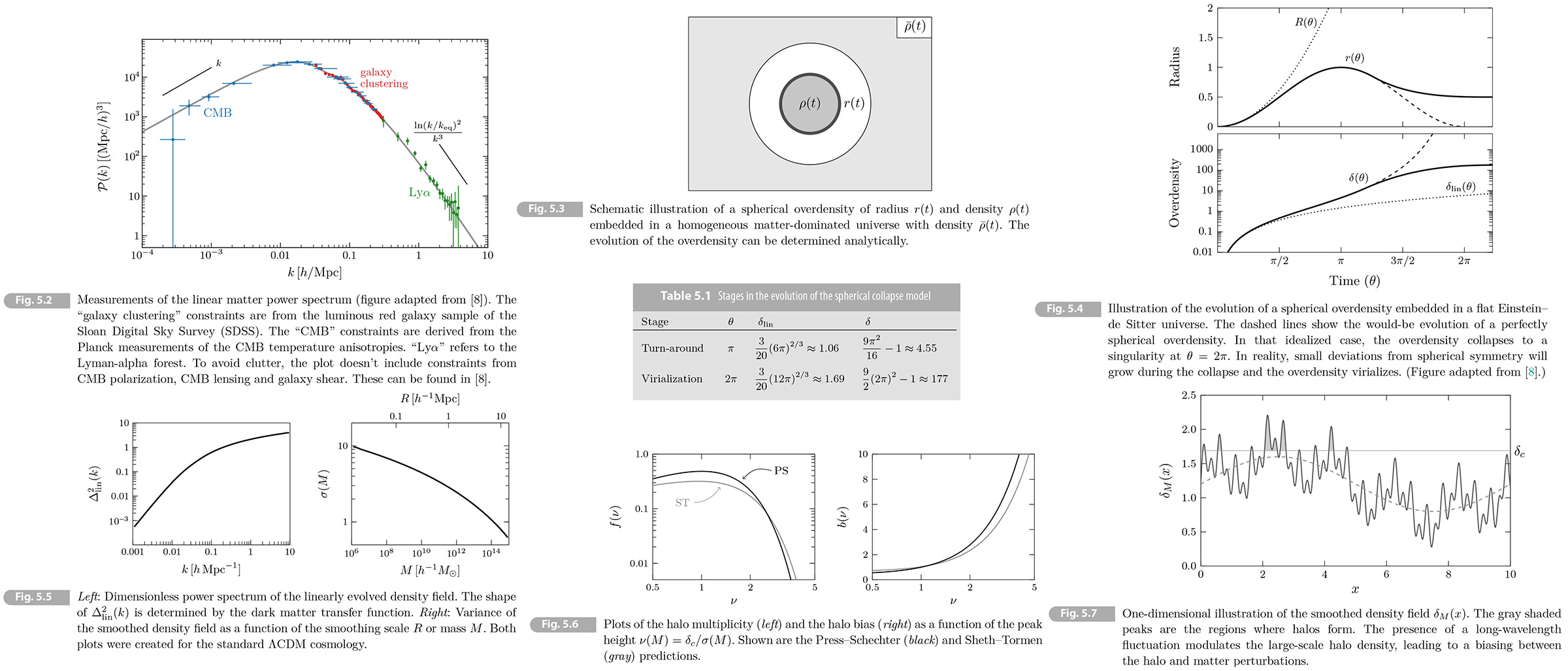
Fig 5.2 shows a compilation of measurements of the linear matter power spectrum, The observed spectrum indeed has the expected asymptotic scalings. On large scale, the measurement comes from observations of the CMB anisotropies. As we will see in Chapter 7, the dark matter perturbations affect the evolution of photon-baryon fluid before recombination, as well as the free-streaming of the photon after decoupling. The latter arises because the fluctuations in the distribution of galaxies are related to fluctuations in the matter through 𝛿𝑔 = 𝑏𝛿, where the parameter 𝑏 is called the galaxy bias. Taking this biasing into account, the galaxy power spectrum becomes a measure of the underlying matter density perturbations.2
Exercise 5.6 Show that
(5.83) 𝑘eq = 𝐻0 √(2𝛺𝑚/𝑎eq) ≈ 0.015 𝘩 Mpc-1,
where the second equality assumes standard values for the cosmological parameters. This explains the position of the turn over in Fig. 5.2.
[Solution] We wish to determine the critical wavenumber at matter-radiation equality, 𝑘eq ≡ 𝑎eq𝐻eq. [RE p.179]
(a-c) 𝐻2 = 𝐻02 (𝛺𝑚𝑎-3 + 𝛺𝑟𝑎-4), 𝑎2𝐻2 = 𝐻02𝛺𝑚/𝑎 (1 + 𝑎eq/𝑎), [with 𝛺𝑟 = 𝑎eq𝛺𝑚 𝑎eq𝐻eq = 𝐻0√(2𝛺𝑚/𝑎eq) = 𝑘eq.
Using 𝐻0 ≈ (2998)-1 𝘩 Mpc-1, [Wikipedia Hubble's law: Dimensionless Hubble constant] 𝛺𝑚 ≈ 0.32 and 𝑎eq ≈ (3400)-1, [Table 2.1] we get
(d) 𝐻0 √(2𝛺𝑚/𝑎eq) ≈ 1/2998 × √(2 × 0.32 × 3400) ≈ 0.016 𝘩 Mpc-1, ▮
Other important tracer of the matter density fluctuations are galaxies. As we will see in Section 5.4.4 galaxies form inside dark matter halos, which itself are created at peaks of the dark matter density field. We will show that the density fluctuations in the distribution of galaxies are related to fluctuations in the matter through 𝛿𝑔 = 𝑏𝛿, where the parameter 𝑏 is called the galaxy bias. Taking this biasing into account, the galaxy power spectrum becomes a measure of the underlying matter power spectrum
(5.84) 𝒫𝑔(𝑘) = 𝑏2𝒫(𝑘).
Note that the bias parameter can be different for different galaxy populations and that it becomes scale dependent when linear theory stops being a good approximation.
5.4 Nonlinear Clustering*
so far, our treatment has been restricted to the linear regime where 𝛿 ≪ 1. To understand the formation of small-scale structures (like galaxies and clusters of galaxies), with 𝛿 ≫ 1, we must go beyond the linearized analysis and tackle the nonlinear regime. This is challenging3 and ultimately requires numerical simulations. We will study a simple toy mode with a high degree of symmetry that provides the nonlinear evolution analytically [7].
5.4.1 Spherical Collapse
Consider a flat, matter-dominated universe. The average density is equal to the critical density and evolve as [RE (2.142), (2.147) and (3.56) when 𝑎 ∝ 𝑡2/3, 𝐻 = 2/3𝑡.]
(5.85) 𝜌̄(𝑡) = 1/6π𝐺 1/𝑡2.
At time 𝑡𝑖, we create a spherically symmetric overdensity by compressing a region of radius 𝑅𝑖 to one with radius 𝑟𝑖 < 𝑅𝑖; see Fig. 5.3. The initial density of the perturbation is
(5.86) 𝜌𝑖 = 𝜌̄𝑖𝑅𝑖3/𝑟𝑖3 ≡ 𝜌̄𝑖(1 + 𝛿𝑖),
where the mass of the compressed region is conserved. As before we introduce the density contrast 𝛿, but this time we will not assume that it stays small throughout the evolution.
We gain a few things from the the spherical symmetry of the situation. First, the evolution of the background will not be affected by the presence of perturbation. Second, the perturbation also evolves independently from the background. Third, we can think of he overdensity as consisting of many distinct mass shells. Our analysis will remain valid as long as these thin shells evolve independently, but breaks down when "shell crossing" occurs.
Let us study the evolution of a single shell of radius 𝑟(𝑡). In Newtonian gravity, the conservation of energy for mass shell reads
(5.87) 1/2 𝑟̇2 - 𝐺𝑀(𝑟)/𝑟 = 𝐸,
where 𝑀(𝑟) is the mass closed by the shell. Both 𝑀(𝑟) and 𝐸 are constant throughout the evolution. In side the overdensity, we have 𝐸 < 0, so that the overdensity acts like a closed universe with positive curvature. In fact, we solved this problem in Section 2.3.6, where we saw that a closed universe initially expands, before recollapsing under thr gravitational attraction of the excess density (cf. Fig. 2.12. The parametric solution for the evolution of the radius of the closed universe was given in (2.169) and (2.170). The solution is of the same form
(5.88) 𝑟(𝜃) = 𝛢(1 - cos 𝜃), 𝑡(𝜃) = 𝛣(𝜃 - sin 𝜃), [verification needed]
(5.89) 𝛢 ≡ 𝐺𝑀/2∣𝐸∣, 𝛣 ≡ 𝐺𝑀/(2∣𝐸∣)3/2, 𝛢3 ≡ 𝐺𝑀𝛣2.
At early times, 𝜃 ≪ 1, we find that
(5.90) 𝑟(𝜃) ≈ 𝛢/2 𝜃2, 𝑡(𝜃) ≈ 𝛣/6 𝜃3 } ⇒ 𝑟(𝑡) ≈ 𝛢/2 (6/𝛣)2/3 𝑡2/3. [verification needed]
Initially the overdense region evolves in the same way as the background, bur eventually the expansion will slow down and the overdense region will collapse just like a closed universe. The time at which the expansion halts is 𝜃turn = π, while the time of collapse is 𝜃col = 2π.
Using (5.88), we find that the density of the perturbation and the density of the background evolve as
(5.91) 𝜌(𝜃) = 𝑀/[(4π/3)𝑟3(𝜃)] = 3𝑀/4π𝛢4 1/(𝜃 - cos 𝜃)3,
(5.92) 𝜌̄(𝜃) = 1/6π𝐺 1/𝑡2(𝜃) = 1/6π𝐺𝛣2 1/(1 - sin 𝜃)2.
The ratio of (5.91) and (5.92) determines the density contrast
(5.93) 1 + 𝛿 = 𝜌/𝜌̄ = 9/2 (𝜃 - sin 𝜃)2/(1 - cos 𝜃)3,
where we used that 𝛢3 ≡ 𝐺𝑀𝛣2. It's useful to consider three distinct stages of the evolution (see Dig. 5.4 and Table 5.1:
• Linear regime At early times, when 𝛿 is still small, we expect this result to recover the solution in linear perturbation theory. Expanding (5.93) for small 𝜃, we get
(5.94) 𝛿 ≈ 3/20 𝜃2 = 3/20 (6/𝛣)2/3 𝑡2/3 ≡ 𝛿lin(𝑡),
which indeed is the expected scaling, 𝛿lin ∝ 𝑎 [∝ 𝑡2/3]. The solution in (5.93) holds even for large 𝛿.
• Turn-around A the turn-around point, we find
(5.95) 𝛿(𝜃turn = π) = 9π2/16 - 1 ≈ 4.55.
It is also useful to ask what the extrapolated linear solution would be at the turn-around point. Using (5.94), we get
(5.96) 𝛿lin(𝑡) = 3/20 (6π)2/3 ⇒ 𝛿lin(𝑡turn) = 3/20 (6π)2/3 ≈ 1.06,
where we used that 𝑡turn = 𝛣π.[verification. needed] Though 𝛿lin(𝑡turn) is a bit of an artificial concept, it provides an easy way to judge by extrapolation of the linear solution whether a region of space should be viewed as decoupled from the Hubble flow.
• Collapse A the collapse time, the solution formally diverges,
(5.97) 𝛿(𝜃col = 2π) = ∞,
signaling a point of infinite density. We will discuss the meaning of divergence in the next section. Let us ask again what the linear solution would be if we extrapolated it to the collapse time. Using 𝑡col = 2𝑡turn = 2𝛣π, we find
(5.98) 𝛿lin(𝑡col) = 3/20 (12π)2/3 ≈ 1.69.
Once a naive extrapolation of linear perturbation theory reaches 𝛿lin = 1.69. we should therefore think of the region as completely collapsed.
5.4.2 Virialization and Halos
The divergence that we found is an artifact of assuming perfect spherical symmetry for the initial perturbation. Such perfect symmetry does not exist in the real world. Instead, any deviation from spherical symmetry will get amplified during the collapse. The individual shells will stop to evolve independently and start crossing. Ultimately, the matter will virialize, meaning that it will settle into equilibrium configuration with balanced kinetic and potential energies. The final object is an extended dark matter halo. These halos are the locations where baryons will eventually cluster into galaxies.
We can use the virial theorem to estimate the density of the dark matter halos. The theorem state that, for virialized objects, the averge kinetic energy, 𝛵 is related to the average potential energy, 𝑉 by
(5.99) 𝛵 = -1/2 𝑉.
We will this with the conservation of energy, 𝐸 = 𝛵 + 𝑉 = const. At the turn-around point, the kinetic energy vanishes and the total energy is 𝐸 = 𝑉turn. After virialization, we then have
(5.100) 𝛵vir + 𝑉vir ⇒ 1/2 𝑉vir = 𝑉turn. [correction: from '=' to '⇒']
this implies hat the radius of the virialized halo is half the radius of the perturbation at turn-around, 𝑟vir = 𝑟turn/2, and the density of halo is 8 times the density at turn-around, 𝜌vir = 8𝜌turn. Let us compare this to the background density at virialization. For simplicity, we take the time of virialization to be the collapse time, 𝑡vir ~ 𝑡col = 2𝑡turn. Since 𝜌̄ ∝ 𝑡-2, this then leads to 𝜌̄ vir = 𝜌̄ turn/4. Assuming all the pieces, the density contrast after virialization is
(5.101) 1 + 𝛿vir = 𝜌vir/𝜌̄ vir = 8𝜌turn/𝜌̄ turn/4 = 32(1 + 𝛿turn) = 18π2 ≈ 178.
where we used (5.95) for 𝛿turn. The expected density of dark matter halos is therefore roughly 200 times greater than the background density. This agrees with the results of numerical simulations.
5.4.3 A Bound on Lambda
It is interesting to extend the spherical collapse model to the case of a universe with dark energy. Whether a spherical overdensity will recollapse will then depend on he size of the cosmological constant. Now we will derive an upper bound on the size of the cosmological constant by demanding that the initial overdensity can form dark matter halos, a necessary requirement for the formation of galaxies and ultimately life itself. Interestingly, the upper bound will be close to the observed value of the cosmological constant [9].
Equation (5.87) now reads
(5.102) 1/2 ṙ2 - 𝐺𝑀/𝑟 - 1/6 𝛬𝑟2 = 𝐸, [citation needed]
where the functional form of the extra term can be understood by going back to our Newtonian derivation of Friedmann equation in Section 2.3.5. In order for a spherical overdensity to turn around and collapse, there must be a time when the velocity of the mass shell vanishes, ṙ = 0. Such a moment only exists if there is a solution 𝑟(𝑡) to the following cubic equation
(5.103) 1/6 𝛬𝑟3 - ∣𝐸∣𝑟 + 𝐺𝑀 = 0.
However, if 𝛬 is too large then this equation doesn't have a solution.
Exercise 5.7 Show that (5. 103) only have a root with 𝑟 > 0 if
(5.104) √𝛬 < (2∣𝐸∣)3/2/3𝐺𝑀 = 1/3𝛣, where 𝛣 was defined in (5.89).
[Solution] Consider the function
(a-b) 𝑓(𝑟) ≡ 1/6 𝛬𝑟3 - ∣𝐸∣𝑟 + 𝐺𝑀. 𝑑/𝑑𝑟 𝑓(𝑟) = 1/2 𝛬𝑟2 - ∣𝐸∣,
so that the critical points are at [𝑑/𝑑𝑟 𝑓(𝑟) = 0] (c) 𝑟*± ≡ ±√(2∣𝐸∣/𝛬).
Since 𝑓(0) > 0, [𝐺𝑀 > 0], the only way for the function is a positive root is if 𝑓(𝑟*+) < 0:
(d) 𝑓(𝑟*+) = 1/6 𝛬 (2∣𝐸∣/𝛬)3/2 - ∣𝐸∣√(2∣𝐸∣/𝛬) + 𝐺𝑀 = -1/3 𝛬(2∣𝐸∣)3/2/√𝛬 + 𝐺𝑀 < 0 ⇒ √𝛬 < (2∣𝐸∣/𝛬)3/2/3𝐺𝑀. ▮
Next, we want to write the bound in (5. 104) for the initial overdensity. At early times, we can use (5.94) [𝛿 ≈ 3/20 (6𝛣)2/3 𝑡2/3]
(5.105) 𝛬 < 0.01 𝛿3/𝑡2. [𝛬 < (1/3𝛣)2 = 1/9 × (3/20)3 × 62 𝛿3/𝑡2 ≈ 0.01 𝛿3/𝑡2]
To quantify this for our universe, we use that density contrast, 𝛿 ≈ 10-3 at the time of last-scattering, 𝑡 ≈ 1013 s (see chapter 7). This then gives 𝛬 < 10-37 s-2, which implies the following bound on the vacuum energy density
(5.106) 𝜌𝛬 = 𝛬/8π𝐺 < 1010 eV m-3.
Rather remarkably, this bound is only a factor 10 larger than the observed size of the vacuum energy.
5.4.4 Press-Schechter Theory
We learned that whenever a density perturbation in linear theory exceeds the threshold 𝛿c = 1.69, a virialized halo with 𝛿vir = 178 will form. This simple fact was exploited by Press and Schechter to develop a theory for the statistics of dark matter halos [10]. The following is a rough sketch of the Press-schechter theory.
Filtered density field
The first step is to introduce a smoothing (or "filtering") of the linearly evolved density field. This means that we remove contributions to he density field below a certain scale 𝑅. We denote the filtered field by 𝛿𝑅(𝐱) ≡ 𝛿(𝐱: 𝑅). The smoothed density field is the average density in a volume of size 𝑅3. At points where the filtered field 𝛿𝑅 exceeds the threshold 𝛿c, we declare a halo of size 𝑅, or mass 𝑀 ~ 𝜌̄𝑅3, to have formed. By thinking about this as a function of the smoothing scale 𝑅, we can drive the mass distribution of these halos.
The smoothed density field is defined as a convolution with a certain window function
(5.107) 𝛿𝑅(𝐱) = ∫ 𝑑3 𝑥' 𝑊(∣𝐱 -𝐱'∣; 𝑅) 𝛿(𝑡, 𝐱').
The choice of window function is not unique and we will work with a simple top-hat function.4
(5.108) 𝑊(𝑘; 𝑅) = { 3/4π𝑅3 𝑟 < 𝑅 ; 0 𝑟 > 𝑅.
The smoothed field is then the average density in spheres of radius 𝑅, around a point 𝐱. The mass associated to each region is 𝑀 = 4π/3 𝑅3 𝜌̄, where 𝜌̄(𝑡) ≡ ⟨𝜌(𝑡, 𝐱)⟩ is the average density. Often this mass scale is used to label the smoothed density field as 𝛿𝑀. Being a convolution in real space, the smoothed density becomes a product in Fourier space, 𝛿𝑅(𝑡, 𝐤) = 𝑊(𝑘; 𝑅) 𝛿(𝑡, 𝐤), where 𝑊(𝑘; 𝑅) is the Fourier transform of the window function.
Exercise 5.8 Show that the Fourier transform of the top-hat filter is
(5.109) 𝑊(𝑘; 𝑅) = 3/(𝑘𝑅)3 [sin (𝑘𝑅) - 𝑘𝑅 cos (𝑘𝑅)],
and that the variance of the smoothed density can be written as
(5.110-1) 𝜎2(𝑡; 𝑅) = ⟨𝛿𝑅2(𝑡, 𝐱)⟩ = ∫ 𝑑 ln 𝑘 ∆lin2(𝑡, 𝑘) ∣𝑊(𝑘; 𝑅)∣2, where ∆lin2(𝑡, 𝑘) ≡ 𝑘3/2π2 𝒫lin(𝑡, 𝑘).
Evaluating this variance for the specific scale 𝑅 = 8𝘩-1 Mpc gives the parameter 𝜎8 which is often used as a measure of the fluctuation amplitude. It measured value today is 𝜎8(𝑡0) ≈ 0.8.
[Solution] The Fourier transform of the top-hat filter is
(a) 𝑊(𝑘; 𝑅) = - ∫ 𝑑3𝑟 𝑒-𝑖𝐤⋅𝐫 𝑊(𝑟; 𝑅) = 2π ∫0𝑅 𝑟2𝑑𝑟 ∫-11 d cos 𝜃 𝑒-𝑖𝑘𝑟 cos 𝜃 3/4π𝑅3 = 3/𝑅3 ∫0𝑅 𝑟2𝑑𝑟 sin 𝑘𝑟/𝑘𝑟 = 3/(𝑘𝑅3)3 [sin(𝑘𝑅) - 𝑘𝑅 cos(𝑘𝑅)].
The coarse-grained field can be written as
(b) 𝛿𝑅(𝑡, 𝐱) = ∫ 𝑑3𝑘/(2π)3 𝑒𝑖𝐤⋅𝐱 𝑊(𝑘; 𝑅) 𝛿(𝑡, 𝐤).
and the variance of the filtered field is
(c) 𝜎(𝑡; 𝑅) ≡ ⟨𝛿𝑅(𝑡, 𝐱)⟩ = ∫ 𝑑3𝑘/(2π)3 ∫ 𝑑3𝑘'/(2π)3 𝑒𝑖(𝐤+𝐤')⋅𝐱 𝑊(𝑘; 𝑅)𝑊(𝑘'; 𝑅) ⟨𝛿(𝑡, 𝐤)𝛿(𝑡, 𝐤')⟩
= ∫ 𝑑3𝑘/(2π)3 ∫ 𝑑3𝑘'/(2π)3 𝑒𝑖(𝐤+𝐤')⋅𝐱 𝑊(𝑘; 𝑅)𝑊(𝑘'; 𝑅) (2π)3 𝛿𝐷(𝐤+𝐤') 𝒫lin(𝑡, 𝑘) [RE (5.72]
= ∫ 𝑑3𝑘/(2π)3 ∣𝑊(𝑘; 𝑅)∣2 𝒫lin(𝑡, 𝑘) = ∫02π 𝑑𝜙 ∫-1+1 𝑑(cos 𝜃) ∫0∞ 𝑑𝑘 𝑘2 ∣𝑊(𝑘; 𝑅)∣2 𝒫lin(𝑡, 𝑘)
= 2π × 2 ∫ 𝑑𝑘/𝑘 ∣𝑊(𝑘; 𝑅)∣2 𝑘3/(2π)3 𝒫lin(𝑡, 𝑘) = ∫ 𝑑 ln 𝑘 ∣𝑊(𝑘; 𝑅)∣2 𝑘3/2π2 𝒫lin(𝑡, 𝑘) = ∫ 𝑑 ln 𝑘 ∣𝑊(𝑘; 𝑅)∣2 ∆lin2(𝑡, 𝑘). ▮
Fig. 5.5 shows the predictions of the standard 𝛬𝐶𝐷𝑀 cosmology for the dimensionless power spectrum of linearly evolved field and variance of the smoothed density field. Over a small range of scales, the linear power spectrum can be written as a power law
(5.112) 𝒫lin(𝑡, 𝑘) = 𝛢𝑘𝑛𝛵2(𝑘) 𝐷+2(𝑡)/𝐷+2(𝑡𝑖) ≡ 𝛢(𝑡)𝑘𝑛eff(𝑘),
where 𝛵(𝑘) is the dark matter transfer function and 𝑛eff(𝑘) is the effective spectral index. Substituting this into (5.110), we find
(5.113) 𝜎(𝑅) ∝ 𝐷+(𝑡) 𝑅(𝑛*eff + 3)/2 𝜎(𝑀) ∝ 𝐷+(𝑡) 𝑀-(𝑛*eff + 3)/6,
where 𝑛*eff(𝑘*) is the spectral index evaluated at 𝑘* = 2π/𝑅. As we see from Fig. 5.5 in a cold dark matter cosmology, we have 𝑛*eff + 3 > 0 and 𝜎(𝑀) is a monotonically decreasing function of mass. Hot dark matter leads to an extra suppression of power on small scales and can therefore give 𝑛*eff + 3 < 0, for large 𝑘*. This qualitative distinction between hot and cold dark matter will become important in a moment.
Mass function
The first statistical quantity that we will discuss is the number of halos in a given mass range. Let 𝑛𝘩(𝑡, 𝐱, 𝑀) be the number of halos of mass 𝑀 at a position 𝐱 and time 𝑡, and 𝑛̄𝘩(𝑡, 𝑀) ≡ ⟨𝑛𝘩(𝑡, 𝐱, 𝑀)⟩ be its mean value. To reduce clutter, I will often suppress the time dependence.
We will assume that the smoothed density is a Gaussian random field. The probability that a region of space has an overdensity 𝛿𝑀 is then given by
(5.114) 𝚸(𝛿𝑀) = 1/√[2π𝜎2(𝑀)] exp [-1/2 𝛿𝑀2/[𝜎2(𝑀)],
where 𝜎2(𝑀) is the variance of the filtered field defined in (5.110). The probability for a region to exceed the density threshold 𝛿c is
(5.115) 𝚸(𝛿𝑀 > 𝛿c) = ∫𝛿c∞ 𝑑𝛿𝑀 𝚸(𝛿𝑀) = ∫𝜈∞ 𝑑𝑥 𝑒-𝑥2/2 = 1/2 erfc(𝜈/√2),
where 𝜈𝑀 ≡ 𝛿c/𝜎(𝑀) is the so-called peak height and erfc(𝑥) is the complementary error function. As we saw in Fig. 5.5, in the standard 𝛬CDM cosmology, the variance 𝜎(𝑀) is a decreasing function of mass 𝑀. This implies that small-scale fluctuations are the first to collapse. This type of structure formation is called "bottom up," because small-scale structures form first and then merge into larger objects. In the once popular hot dark matter models, structure would instead form in a "top down" fashion.
There is a problem with the result in (5.115). In the limit 𝑅 → 0, it should give the fraction of all mass n virialized objects. However, since 𝜎(𝑅) → ∞ in this limit and erfc(0) = 1, the answer in (5.115) implies that only half of the mass collapses into halos. The problem arises because only overdense regions, with 𝚸(𝛿𝑀 > 0) = 1/2, ends up in collapsed objects. Press and Schechter "solved" this so-called cloud-in-cloud problem by multiplying the result by a factor two, 𝚸̄ ≡ 2𝚸, but the justification wan't very satisfactory. Later Bond, Cole, Efstathiou and Kaiser [12] introduced an extension using excursion set theory.5 The final result for the mass functions is the same, so we will proceed with the simpler analysis.
Given (5.115), the probability that a halo formed in the range [𝑀, 𝑀 + 𝑑𝑀] is
(5.116) 𝑃([𝑀, 𝑀 + 𝑑𝑀]) = ∣𝚸̄(𝛿𝑀 + 𝑑𝑀 > 𝛿c) - 𝚸̄(𝛿𝑀 > 𝛿c)∣ ≈ 𝑑𝚸̄/𝑑𝑀.
The abundance of halos of mass 𝑀, the mass function is obtained by multiplying this by the maximum number density of such halos in a region of mean density 𝜌̄ as follows
(5.117) 𝑑𝑛̄𝘩/𝑑𝑀 = -𝜌̄/𝑀 𝑑𝚸̄/𝑑𝑀 = -√(2/π) 𝜈 exp [-𝜈2/2] 𝜌̄/𝑀2 (𝑑 ln 𝜎)/(𝑑 ln 𝑀).
For small 𝜈 the mass function is a power law, while for large 𝜈 it has an exponential fall-off. The function of the peak height 𝜈 in (5.117) is called the halo multiplicity
(5.118) 𝑓PS(𝜈) ≡ √(2/π) 𝜈 exp [-𝜈2/2].
Although that Press-Schechter mass function capture essential qualitative features of halo formation, wuch as the exponential suppression at large mass, it disagrees with the results of N-body simulations at quantitative level. In underpredicts the abundance of rare high-mass halos by factor 10 and overpredicts that of low-mass halo by factor 2. However the Press-Schechter treatment is still remarkable that it captures the correct shape and overall normalization of mass function, It was the starting point for many more precise theories of halo formation [11, 13].
Exercise 5.9 Using (5.113) show that the Press-Schechter mass function can be written as
(5.119) 𝑑𝑛̄𝘩/𝑑𝑀 ≈ 𝛾 𝛽(𝑡)/√π 𝜌̄/𝑀2 𝑀𝛾/2 exp(-𝛽2(𝑡)𝑀𝛾),
where 𝛾(𝑀) ≡ 1 + 𝑛̄eff(𝑀)/3.
[Solution] The variance of the smoothed density is from (5.113)
(a) 𝜎(𝑡; 𝑀) ∝ 𝐷+(𝑡)𝑀-𝛾/2 ⇒ (𝑑 ln 𝜎)/(𝑑 ln 𝑀) = -𝛾/2
where 𝛾 ≡ 1 + 𝑛̄eff/3. The peak height 𝑣(𝑀) = 𝛿c/𝜎(𝑀) = 𝛿c/𝐷+(𝑡) 𝑀𝛾/2 ≡ √2 𝛽(𝑡) 𝑀𝛾/2, and from (5.117) we get
(b) 𝑑𝑛̄𝘩/𝑑𝑀 = -√(2/π) 𝜈 exp [-𝜈2/2] 𝜌̄/𝑀2 (𝑑 ln 𝜎)/(𝑑 ln 𝑀) = -√(2/π) √2 𝛽(𝑡) 𝑀𝛾/2 𝜌̄/𝑀2 ( -𝛾/2) exp [-𝛽2(𝑡) 𝑀𝛾]
= 𝛾 𝛽(𝑡)/√π 𝜌̄/𝑀2 exp [-𝛽2(𝑡) 𝑀𝛾]. ▮
Inspired by the the Press-Schechter mass function, Sheth and Tormen proposed a fitiing function which could be tuned to allow for a better agreement with N-body simulation [14]
(5.120) 𝑓ST(𝜈) ≡ 𝛢√(1/π) [1 + (𝑎𝜈2)-𝑝] √(𝑎𝜈2) exp [-𝑎𝜈2/2],
where 𝛢 =0.32, 𝑎 = 0.75 and 𝑝 = 0.3 to match simulations. Fig. 5.6 shows a comparison between the Press-Schechter and Sheth-Tormen predictions.
Biasing
The mass function tells us how many halos of a given mass 𝑀. Next we would like to determine how these halos are distributed in the volume. We want to compute the correlations in the primordial density field. We define the density contrast of halos as
(5.121) 𝛿𝘩(𝐱; 𝑀) ≡ [𝑛̄𝘩(𝐱; 𝑀) - 𝑛̄̄𝘩(𝑀)]/𝑛̄̄𝘩(𝑀),
and the corresponding two-point correlation function is
(5.122) 𝜉𝘩𝘩(𝑟; 𝑀) = ⟨𝛿𝘩(𝐱; 𝑀)𝛿𝘩(𝐱 + 𝐫; 𝑀)⟩.
Our task is to relate 𝜉𝘩𝘩 to the two-point function of the linear density field 𝜉lin. The simplist way to do this uses the so-called peak background split [15-18]. Let us separate a density perturbation into a short-wavelength part ("peaks"), 𝛿𝘩, and a long-wavelength part ("background"), 𝛿𝑏, so that
(5.123) 𝛿 = 𝛿𝘩 + 𝛿𝑏.
The peaks will eventually form halos, while the long-wavelength fluctuations modulate the local conditions for this halo formation. Since 𝛿𝑏 ≪ 1, the latter can be treated in linear theory. We can assume that 𝛿𝑏 is essentially constant over the scales that 𝛿𝘩 collapses into halos. The long-wavelength perturbation then affects the halo formation in two ways:
• First, it shifts the background density seen by the peaks to
(5.124) 𝜌̄' = 𝜌̄(1 + 𝛿𝑏).
• Second, it perturb the threshold for halo collapse. The linear part of 𝛿𝘩 now forms a halo when it reaches the effective threshold
(5.125) 𝛿𝑐' = 𝛿𝑐 - 𝛿𝑏,
corresponding to the original threshold 𝛿𝑐 for the total density perturbation 𝛿. Since the effective threshold 𝛿𝑐' depends on the value of the long-wavelength fluctuation 𝛿𝑏, the local number density of halos becomes modulated by the field 𝛿𝑏. In regions with positive 𝛿𝑏 halos forms earlier than in regions with negative 𝛿𝑏. The effect is illustrated in Fig. 5.7.
Expanding the mass function to linear order in 𝛿𝑏, we get
(5.126) 𝑑𝑛𝘩/𝑑𝑀 (𝛿𝑏) = 𝑑𝑛̄𝘩/𝑑𝑀 + [∂/∂𝜌̄' (𝑑𝑛̄𝘩/𝑑𝑀) 𝑑𝜌̄'/𝑑𝛿𝑏 + ∂/∂𝛿𝑐' (𝑑𝑛̄𝘩/𝑑𝑀) 𝑑𝛿𝑐'/𝑑𝛿𝑏]𝛿𝑏
= 𝑑𝑛̄𝘩/𝑑𝑀 [1 + (𝜌̄ ∂/∂𝜌̄' ln (𝑑𝑛̄𝘩/𝑑𝑀) - ∂/∂𝛿𝑐' ln (𝑑𝑛̄𝘩/𝑑𝑀))𝛿𝑏]. [verification needed]
Using (5.117) we have
(5.127) 𝜌̄ ∂/∂𝜌̄' ln (𝑑𝑛̄𝘩/𝑑𝑀) = 𝜌̄/𝜌̄' = 1/(1 + 𝛿𝑏) ≈ 1, [verification needed]
(5.128) - ∂/∂𝛿𝑐' ln (𝑑𝑛̄𝘩/𝑑𝑀) = - 1/𝜎(𝑀) (𝑑 ln 𝑓(𝜈))/𝑑𝜈 = (𝜈2 - 1)/𝛿𝑐, [verification needed]
where we used the Press-Schechter multiplicity function in the final equality. Equation (5.126) then becomes
(5.129) 𝑑𝑛𝘩/𝑑𝑀 (𝛿𝑏) = 𝑑𝑛̄𝘩/𝑑𝑀 [1 + {1 + (𝜈2 - 1)/𝛿𝑐}𝛿𝑏],
and substituting this into (5.121), we find
(5.130) 𝛿𝘩(𝐱; 𝑀) = [1 + (𝜈2 - 1)/𝛿𝑐]𝛿𝑏(𝐱).
The factor relating 𝛿𝘩 and 𝛿𝑏 is called the linear bias:
(5.131) 𝑏PS(𝜈) = 1 + (𝜈2 - 1)/𝛿𝑐.
This result applies to scales on which the long-wavelength mode can be treated in linear theory, so that the Talyor expansion in (5.129) is a good approximation. On small scales, nonlinear corrections are important and the biasing becomes more complicated [19].
Exercise 5.10 Repeating the above analysis for the Sheth-Tormen mass function (5.120), show that bias parameter is
(5.132) 𝑏ST(𝜈) = 1 + (𝑎𝜈2 - 1)/𝛿𝑐 + 2𝑝/𝛿𝑐[1 + (𝑎𝜈2)𝑝].
A comparison between the bias parameters from the Press-Schechter and Sheth-Torman mass functions is shown in Fig. 5.6.
[Solution] Following the analysis in the above, we have
(a) 𝑑𝑛𝘩/𝑑𝑀 (𝛿𝑏) = 𝑑𝑛̄𝘩/𝑑𝑀 + [∂/∂𝜌̄' (𝑑𝑛̄𝘩/𝑑𝑀) 𝑑𝜌̄'/𝑑𝛿𝑏 + ∂/∂𝛿𝑐' (𝑑𝑛̄𝘩/𝑑𝑀) 𝑑𝛿𝑐'/𝑑𝛿𝑏]𝛿𝑏
= 𝑑𝑛̄𝘩/𝑑𝑀 [1 + (𝜌̄ ∂/∂𝜌̄' ln (𝑑𝑛̄𝘩/𝑑𝑀) - ∂/∂𝛿𝑐' ln (𝑑𝑛̄𝘩/𝑑𝑀))𝛿𝑏] = 𝑑𝑛̄𝘩/𝑑𝑀 [1 + {1 - 𝜈/𝛿𝑐 (𝑑 ln 𝑓(𝜈))/𝑑𝜈}𝛿𝑏],
and the bias parameter is, (b) 𝑏(𝜈) = 1 - 𝜈/𝛿𝑐 (𝑑 ln 𝑓(𝜈))/𝑑𝜈.
For the Sheth-Torman function (5.120), 𝑓ST(𝜈) ≡ 𝛢√(1/π) [1 + (𝑎𝜈2)-𝑝] √(𝑎𝜈2) exp [-𝑎𝜈2/2], we get, as required
(c) 𝑏ST(𝜈) = 1 + (𝑎𝜈2 - 1)/𝛿𝑐 + 2𝑝/𝛿𝑐[1 + (𝑎𝜈2)𝑝]. ▮
Given (5.130), the halo two-point function can be written as
(5.133) 𝜉𝘩𝘩(𝑟; 𝑀) = 𝑏2(𝑀) 𝜉lin(𝑟),
where 𝜉lin(𝑟) is the dark matter two-point function predicted in linear perturbation theory. We say the dark matter halos are "niasestracers" of the underlying density field. Since 𝑏(𝑀) is a monotonically increasing function, the biasing is stronger for more massive halos. Finally, because galaxies form inside of dark matter halos, the halo correlations are closely related to the observed galaxy correlations, and an ansatz like (5.133) is also used for the galaxy two-point function 𝜉𝑔𝑔(𝑟).
2 The matter perturbations also affect the observed CMB fluctuations through gravitational lensing. For clarity in Fig. 5.2 these lensing and constraint from galaxy shear. The full set of constraint is in [6]. There it is also explained how the measurements of the nonlinear power spectrum are related back to the linear power spectrum at 𝑧 = 0.
3 Three apparent complications are i) Different Fourier modes start to couple to each other; ii) the evolution cannot be described by a simple growth function iii) the density field becomes non-Gaussian.
4 The drawback of this window function is that the sharp edge at 𝑟 = 𝑅 create power on all scales in Fourier space. Sometimes the window function is defined as a sharp cut-off in Fourier space, with 𝑊(𝑘; 𝑅) = 1 for 𝑘𝑅 < 1 and 0 otherwise. This has the disadvantage that there isn't a well-defined volume associated to the window function. A compromise is a Gaussian window function which has a smooth cut-off in both position and momentum space.
5 The idea is to consider the density field 𝛿𝑅 as a function of smoothing scale 𝑅. At a fixed location this produces a curve that looks like a random walk staring at 𝛿𝑅 = 0 for 𝑅 → ∞. The cloud-in-cloud problem is solved by identifying a halo with the largest smoothing scale at which the random walk first crosses the threshold 𝛿c for collapse, which removes the double-counting of smaller halos from the problem.
|
|
|