|
김관석
|
2025-01-08 22:13:54, 조회수 : 38 |
- Download #1 : BC_8d.jpg (545.5 KB), Download : 0

8.4 Observational Constraints*
In the previous sections, we showed that inflation contains a built-in mechanism to produce a nearby scale-invariant spectrum of primordial curvature perturbations. In this section the current observational evidence for inflation will be described and future observational tests will be discussed.
8.4.1 Current Results
It is remarkable that we now have observations that probe the physical conditions just fractions of a second after the Big Bang, when the energies were many orders of magnitude higher than the highest energies accessible to particle colliders. In this following, what we have learned from these observations will be explained.
Scale invariance
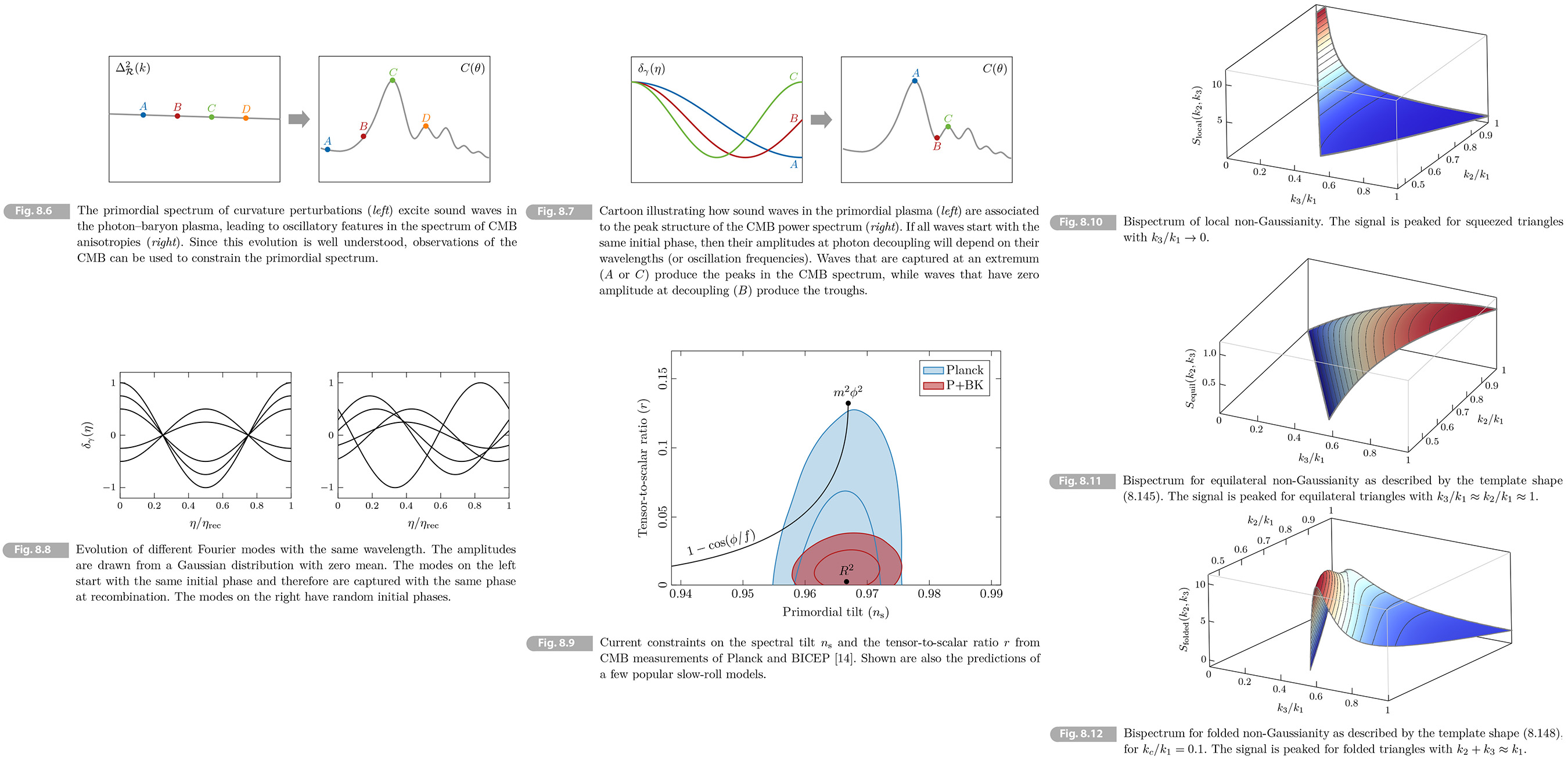
As we saw in Chapter 7, the main feature of the CMB spectrum arise from the evolution of coupled photon-baryon fluctuations on subhorizon scales. We found that a nearby featureless spectrum of initial fluctuations evolves into the peaks and troughs of the CMB anisotropy spectrum (see Fig. 8.6. Since the evolution of the fluctuations after inflation is well understood, we can use the CMB observations to put constraonts on the primordial power spectrum and hence on the physics of inflation.
A key prediction of inflation is the fact that the primordial correlations are approximately scale invariant, corresponding to the approximate time-translation invariance of the the inflationary dynamics. Inflation also predicts a percent-level deviation from perfect scale invariance arising from the small time dependence that is required because inflation has to end. This breaking of perfect scale invariance was measured by the WMAP and Plank satellites. The latest measurement of the scalar spectral index is [3]
(8.135) 𝑛𝑠 = 0.9652 ± 0.0042,
which deviates at a stastically significant level from 𝑛𝑠 =1. The sign of the deviation, 𝑛𝑠 < 1, is also what would be expected from a decreasing energy density during inflation.
Coherent phases
Possibly the most remarkable evidence for inflation come from the phase coherence of the primordial fluctuations. If the perturbations in photon-baryon fluid didn't have coherent phases, then the sound waves in the plasma wouldn't interfere constructively at recombination and the CMB power spectrum would not have its famous peak structure. It will now be explained why this phase cohereence arises naturally in inflationary models. A more detailed version of the smae argument has appeared in a nice article by Dodelson [9].
The CMB is a snapshot of sound waves at the time of recombination (or more precisely photon decoupling). Each wave is captured at a certain phase in its evolution (see Fig. 8.7). Since the oscillation frequency is set by the wavelength of the wave, 𝜔 = 𝑐𝑠𝑘, waves with different wavelengths are observed at different moments in their evolution. This is the reason why the angular power spectrum of the temperature fluctuations goes up and down as a function of scale. While this cartoon is essentially correct, it doesn't highlight the fact that the initial phases must be synchronized. Even a single Fourier mode should be of as an ensemble of many waves with fixed wavelength, but amplitudes that are drawn from a Gaussian probability distribution. These waves need to be added to get the real space density distribution and hence the CMB anisotropies. The modes will only have the same phase at recombination if their initial phases are the same (see Fig. 8.8). Thhis coherence of the phase is necessary in order for the superposition of many modes to lead to the peak structure seen in the CMB spectrum. If the initial phase were random, then the peaks of the spectrum would be washed out.
In inflation, the initial phases are set by the fact that the modes are frozen noutside of the horizon. When the modes re-enter the horizon, the time derivative of the amplitude, 𝓡ʹ, is small. All modes with the same wavenumber 𝑘, but distinct wavevectors 𝐤, therefore start their evolution at the sametime. Thinking of the Fourier modes as a combination of sine and cosine solutions, inflation only excites the cosine solution. What is remarkable is that the coherence of the phases extends to superhorizon scales at recombination. This is seen most convincingly in the ctross correlation between fluctuations in the CMB temperature and E-mode polarization. Since polarization is generated only by scattering of the photons off the free electrons just before decoupling, this signal cannot be created after recombination. Without inflation (or smething very similar), such a signal would causality [10]. The large-scale TE(temperature-E mode) correlation signal was detected for the first time by the WMAP satellite [11].
Adiabaticity
In Section 6.2 we showed that the most general initial conditions for the fluid components of the hot Big bang may include isocurvature contributions. However, these isocurvature fluctuations are not a natural outcome of the simplest inflationary models. Instead, single-field inflation has only one fluctuating scalar degree of freedom, which induces purely adiabatic initial conditions. Moreover, thermal equilibrium after inflation tends to wash out any isocurvature modes.
The peak structure of the CMB spectrum is evidence that the dominant contribution to the primordial perturbations is adiabatic. As we have seen, adiabatic initial conditions produce a cosine oscillation in the photon-baryon plasma. Isovurvature initial conditions, on the other hand, would create a sine oscillation which is not consistent with the observed peaks of the CMB. The possibility of a dominant isocurvature perturbation is ruled out and even a subdominant level of isocurvature fluctuations is highly constrained.
Observational constraints on isocurvature modes depend on whether they are correlated or uncorrelated with the adiabatic mode. In the totally correlated case, all fluctuations are still proportional to 𝓡and we cawrite the matter isocurvature mode as
(8.136) 𝑆𝑚 = √𝛼 𝓡.
The Planck limit on the proportionality constant is [12]
(8.137) 𝛼 < 0.0003+0.0016-0.0012.
A more detailed analysis for CDM, neutrino density and neutrino velocity isocurvature modes gives similar results. There is, hence, no evidence for any isocurvature contribution to the initial perturbations, in agreement with the expectation from single-field inflation.
Gaussianity
So far, we have only described constraints arising from the two-point function of the primordial correlations. This two-point function, in fact, contains all the information about the initial conditions if the perturbations are drwan from a Gaussian probability distribution. The simplestinflationary models indeed predict Gaussanity to be a good approximation. It is easy to see why. Slow-roll inflation only occurs on the flat part of the potential where the self-interactions of the field are small. The linearized equation of motion is then a good apporoximation for the evolution of the inflaton fluctuations. This equation took the form of a harmonic oscillator equation, which we used to compute the expectation value of quantum fluctuations in the ground states. Since the ground state wave function of the harmonic oscillator is a Gaussian, we expect the initial perturbations created by inflation also to obey Gaussian statistics. All odd 𝑁-point functions then vanish, while all even 𝑁-point functions are related to the power spectrum (which contains all the information).
Small amounts of non-Gaussianity may nevertheless still exist and would teach us a lot about the physics of inflation. In particular, extentions of slow-roll modes can produce non-Gaussian fluctuations from enhanced self-interactions of the inflaton or couplings to additional fields. Below the current constraints and future tests of these types of non-Gaussianity.
8.4.2 Future Tests
Although the evidence for inflation is intrigging, we cannot yet claim that it is part of the standard model of cosmology at the same level as, for example, BBN and/or recombination are. Since unlike them inflation requires physics beyond the Standard Model of particle physics. We need further observational tests. In this section, two avenues that are considered particularly promising: tensor mode and non-Gaussianity will be mentioned.
Tensor modes
A major goal of current efforts in observational cosmology is to detect the tensor component of the primordial fluctuations. As we saw, the tensor amplitude depends on the energy scale of inflation and is therefore nor predicted (i.e. it varies between models). While this makes the search for primordial tensor modes difficult, it is also what makes it exciting. Detecting tensors would reveal the energy scale at which inflation occurred, providing an importan clue about the physics driving the inflationary expansion. As in Section 8.3,2 the tensor signal is also unusually sensitive to high-energy corrections and therefore probes important aspects the microphysics of inflation and the nature of quantum gravity [1].
Most searches for tensor modes focus on their imprint on the polarization of the CMB. As in Chapter 7 polarization is generatedthrough the scattering of the anisotropic radiation field off the free electons just before decoupling. The presence of a gravitational wave background creates an anisotropic stretching of the spacetime which induces a special type of polarization pattern, the so-called B-mode pattern ( a pattern whose "curl" doesn't vanish). Such a pattern cannot be created by scalar fluctuations and is therefore a unique signature of primordial tensors. Because tensors are such a clean prediction of inflation, a B-mode detection would be a milestone towards establishing that inflation really occurred in the early universe.
The latest observational constraints are shown in Fig. 8.9. implying an upper bound on the tensor-to-scalar ratio of 𝑟 < 0.035 [13]. A large number of ground-based, balloon and satellite experiments are searching for B-mode signal predicted by inflation (see e.g. [14]). The main challenge for these experiments is to isolate the primordial signal from secondary B-modes created by astrophysical foregrounds. This can be done by using the frequency dependence of the signal (the primordial signal is a blackbody) and the spatial dependence (the primordial signal is statistically isotropic).
Non-Gaussianity
We have seen that inflation predicts that the initial correlations are highly Gaussian and therefore described well by the power spectrum. Nevertheless, in principle, a significant amount of information about the physics of inflation can be coded in small levels of non-Gaussianity. In particular, the higher-order correlations associate with non-Gaussian initial conditions are sensitive to nonlinear interactions, while the power spectrum only probes the free theory. Measurements of primordial non-Gaussian would probe the particle content and the interactions during inflation.3
The leading signature of non-Gaussianity is a nonero thre-point correlation function, or its Fourier equivalent, the bispectrum: [RE Wikipedia Bispectrum]
(8.138) ⟨𝓡𝐤1 𝓡𝐤2 𝓡𝐤3⟩ = (2π)3 𝛿𝐷(𝐤1 + 𝐤2 + 𝐤3) (2π2)2/(𝑘1𝑘2𝑘3)2 𝛣𝓡(𝑘1, 𝑘2, 𝑘3),
where the delta function is a consequence of the homogeneity of the background. The sum of the wavevectors must form a closed triangle and the strength of the signal will depend on the shape of the triangle. The bispectrum is a function of the magnitudes of the wavevectors, 𝑘𝑛=1,2,3, as required by the isotropy of the background. The factor of (𝑘1𝑘2𝑘3)-2 has been extracted in (8.138) to make the function 𝛣𝓡(𝑘1, 𝑘2, 𝑘3) dimensionless. The amplitude of the non-Gaussianity is then defined as the size of the bispectrum in the equilateral configuration:
(8.139) 𝑓𝛮𝐿(𝑘) ≡ - 5/18 𝛣𝓡(𝑘1, 𝑘2, 𝑘3)/∆4𝓡(𝑘),
where the numerical factor is a historical accident and the overall minus sign is a consequence of Baumann's convenstion for sign of 𝓡 (which is different from that used in the Planck and WMAP analysis). In general, the parameter 𝑓𝛮𝐿 can depend on the overall wavenumber (or the size of the triangle), but for scale-invariant initial conditions it would be a constant. Then the bispectrum can be written as
(8.140) 𝛣𝓡(𝑘1, 𝑘2, 𝑘3) ≡ -18/5 𝑓𝛮𝐿(𝑘) × 𝑆(𝑥2, 𝑥3) × ∆4𝓡,
where 𝑥2 ≡ 𝑘2/𝑘1 and 𝑥3 ≡ 𝑘3/𝑘1.4 The shape function 𝑆(𝑥2, 𝑥3) is normalized so that 𝑆(1, 1) ≡ 1. The shape of the non-Gaussianity contains lots of information about the microphysics of inflation. This is to be contrasted with the power spectrum, which described by just two numbers, 𝛢𝑠 and 𝑛𝑠, and not a whole function.
In the following, a mostly qualitative discussion of popular forms of non-Gaussianinty. Further details and explicit computations can be found in [16, 17].
• Local non-Gaussianity One way to create a non-Gaussian field is to take a Gaussian one and add to it the square of itself [18, 19]:5
(8.141) 𝓡(𝐱) = 𝓡𝑔(𝐱) - 3/5 𝑓local𝛮𝐿 [𝓡2𝑔(𝐱) - ⟨𝓡2𝑔 ⟩].
This local field redefinition creates the so-called local non-Gaussianity. The corresponding bispectrum, and the associated shape function, are
(8.142) 𝛣local𝓡 ∝ (𝑘1𝑘2𝑘3)2 (𝒫1𝒫2 + 𝒫1𝒫3 + 𝒫2𝒫3), 𝑆local = 1/3 (𝑘32/𝑘1𝑘2 + 𝑘22/𝑘1𝑘3 + 𝑘12/𝑘2𝑘3),
where 𝒫𝑛 ≡ 𝒫𝓡(𝑘𝑛) and the result for 𝑆local is a scale-invariant power spectrum, 𝒫𝑛 ∝ 𝑘𝑛-3. The shape of the local bispectrum is shown in Fig. 8.10. We see the signal is peaked in the "squeezed limit." where one side of the triangle is much smaller than the other two (say 𝑘3 ≪ 𝑘2 ≈ 𝑘1). Interestingly, this feature cnnot arise in single-field inflation because of the single-field consistency relation [20, 21]. This theorem states that, for any sigle-field model of inflation, the signal in the squeezed limit must satisfy
(8.143) lim𝑘3→0 𝛣local𝓡(𝑘1, 𝑘2, 𝑘3) = (𝑛𝑠 - 1) (𝑘1𝑘2𝑘3)2/(2π2)2 𝒫𝓡(𝑘3)𝒫𝓡(𝑘1),
which vanishes for scale-invariant fluctuations. Therefore detecting a signal in the squeezed limit would rule out all models of single-field inflation. with Bunch Davis initial conditions), not just slow-roll models. Conversely, the signal in the squeezed limit can be used as a particular clean diagnostic for extra fields during inflation. Because inflation occurred at very high energies, even very massive particles (𝑚 ≲ 𝐻) can be produced by the rapid expansion of the spacetime [15, 22]. When these particles decay into the inflaton, they can find to a distinct signature in the squeezed limit of the bispectrum.Planck constraint on local non-Gaussianity is [23]
(8.144) 𝑓local𝛮𝐿 = -0.9 ± 5.1.
Future galaxy survey may improve the bound by an order of magnitude [24], providing a sensitive probe of the particle spectrum during inflation. These measurements exploit the fact that local non-Gaussianity leads to a scale-dependent bias [25] on large scales, which can be measured in the galaxy power spectrum.
• Equilaterial non-Gaussianity In slow-roll inflation the flatness of the inflation potential constrains the size of the inflation self-interactions. However interesting models of inflation have been suggested in which higher derivative corrections-such as (∂𝜙)4-play an important role during inflation [26, 27]. These inflation leads to cubic interactions of the curvature perturbations-such as (d𝓡/d𝑡)3 and (d𝓡/d𝑡)(∂𝑡𝓡)2-and hence a nonzero bispectrum.6 A key characteristic of derivative interactions is that they are suppressed when any individual mode is far outside the horizon. This suggests that the bispectrum is small in the squeezed limit and maximal when all three modes have wavelengths equal to the horizon size. Therefore the bispectrum has a shape that peaks for an equilaterial triangle configuration (𝑘1 ≈ 𝑘2 ≈ 𝑘3).
The precise shape of this equilaterial non-Gaussianity depends on the specific cubic interactions from which it arises; for example, the shapes coming from (d𝓡/d𝑡)3 and (d𝓡/d𝑡)(∂𝑡𝓡)2 are slightly different away from the equilateral limit. The CMB data is typically analyzed using the following template shape [28]:
(8.145) 𝑆equil = - (𝑘12/𝑘2𝑘3 + 2 perms) + (𝑘1/𝑘2 + 5 perms) - 2,
which is plotted in Fig. 8.11. This template is a good approximation to all forms of equilateral non-Gaussianity near the equilateral limit, which is where most of the constraining power of the CMB data comes from. When using other data sets, however, it's important to remember that the template (8.145) is only an approximation. For example, the exact bispectrum coming from the interaction (d𝓡/d𝑡)3 is [27]
(8.146) 𝑆(d𝓡/d𝑡)3 = 27𝑘1𝑘2𝑘3/(𝑘1 + 𝑘2 + 𝑘3)3,
which agrees with (8.145) in the equilaterial configuration, but differs away from it.
Using the template shape (8.145), the planck collaboration derived the following constraint on equilateral non-Gaussianity [23]the secondary non-Gaussianity produced by late
(8.147) 𝑓local𝛮𝐿 = -26 ± 47.
It will be hard (but not impossible) to improve on this constraint with future galaxy surveys, because gravitational nonlinearities also produce an equilateral signal. This makes it challenging to distinguish the primordial non-Gaussianity from the secondary non-Gaussianity produced by the late-time evolution of the perturbations.
• Folded non-Gaussianity The Gaussianity of slow-roll inflation also relies on the fact that we evaluated the quantum fluctuations in the Bunch-Davis vacuum (corresponding to the ground stae of the harmonic oscillator). In contrast, starting from an excited initial state would lead to non-Gaussianity. The detailed shape of this non-Gaussianity, and hence the onstraint on 𝑓𝛮𝐿, depends on the model for the excited initial state [27, 29]. A universal feature is that the correlations are enhanced for "folded" triangles where two of the wavevectors become colinear.
A template that captures the essential features of non-Gaussianity from excited initial states is [16]
(8.148) 𝑆folded ∝ 𝑘12𝑘3 (-𝑘1 + 2 + 𝑘3)/(𝑘𝑐 - 𝑘1 + 𝑘2 + 𝑘3)4 + 2 perms,
where 𝑘𝑐 is a cutoff that regulates the singularity in the folded limit, 𝑘2 + 𝑘3 → 𝑘1. This shape is plotted in Fig. 8.12. Ignoring the cutoff 𝑘𝑐, the function in (8.148) is almost the same as that in (8.146), except for a flipped sign in front of one of the wavenumbers ("energies"). This sign flip arise because an excited initial state contains an admixture of the negative-frequency solution 𝑒+𝑖𝑘𝑛. The alternating signs in (8.148) arises when correlating positive- and negative-frequency modes. It is these alternating signs that are the origin of the enhanced signal in the folded limit.
The signal in the folded configuration also provides an interesting test of the quantum origin of the fluctuations [30] While classical fluctuations would generally have non-vanishing correlations in the folded limit, quantum fluctuations in the Bunch-Davis vacuum are characterized by the absence of such a signal.
8.5 Summary
In this chapter, we have studied the initial fluctuations created by inflation. We showed how quantum zero-point fluctuations get stretched outside the horizon during inflation, becoming the seeds for the large-scale structures of the universe.
We stared by deriving the equation for the inflation fluctuations. In spatially flat gauge, the equation for 𝑓 ≡ 𝑎𝛿𝜙 takes the form
(8.149) 𝑓ʺ + (𝑘2 - 𝑧ʺ/𝑧) 𝑓 = 0, where 𝑧 ≡ 𝑎𝜙̄ʹ/𝓗.
The comoving curvature perturbation is 𝓡 = 𝑓/𝑧. The field 𝑓 and its conjugate momentum 𝜋 ≡ 𝑓ʹ are promoted to quantum operators which satisfy the equal time commutation relation
(8.150) [𝑓̂(𝜂, 𝐱), 𝜋̂(𝜂, 𝐱ʹ)] = 𝑖 𝛿𝐷(𝐱 - 𝐱ʹ).
The field operator is then written as
(8.151) 𝑓̂(𝜂, 𝐱) = ∫ d3𝑘/(2π)3 [𝑓𝑘(𝜂) 𝑎̂𝐤 𝑒𝑖𝐤⋅𝐱 + 𝑓𝑘*(𝜂) 𝑎̂†𝐤 𝑒-𝑖𝐤⋅𝐱],
where 𝑎̂𝐤 and 𝑎̂†𝐤 are annihilation and creation operators, which obey
(8.152) [𝑎̂𝐤, 𝑎̂†𝐤ʹ] = (2π)3𝛿𝐷(𝐤 - 𝐤ʹ).
The vacuum state ∣0⟩ is the state annihilated by 𝑎̂𝐤. A preferred initial state-the Bunch-Davis boundary vacuum-is defined by the ground state of a harmonic oscillator. With this boundary condition, and assuming a de Sitter background, the mode function in (8.151) becomes
(8.153) 𝑓𝑘(𝜂) = 𝑒-𝑖𝑘𝜂/√(2𝑘) (1 - 𝑖/𝑘𝜂).
Using this, the dimensionless power spectrum of the inflaton fluctuation is
(8.154) ∆2𝛿𝜙(𝑘, 𝜂) = 𝑘3/2π2 ∣𝑓𝑘(𝜂)∣2/𝑎2(𝜂) = (𝐻/2π)2 [1 + (𝑘𝜂)2] 𝑘𝜂→0→ (𝐻/2π)2.
The power spectrum of the curvature perturbation 𝓡 takes a power law form
(8.155) ∆2𝓡(𝑘) = 𝛢𝑠 (𝑘/𝑘*)𝑛𝑠 - 1,
where the amplitude and the spectral index are
(8.156) 𝛢𝑠 ≡ 1/8π2 1/𝜀* 𝐻*2/𝑀𝑃𝑙2,
(8.157) 𝑛𝑠 ≡ 1 - 2𝜀* - 𝜅*.
All quantities on the right side are evaluated at the time when the reference scale 𝑘* exited the horizon, 𝑘* = (𝑎𝐻)*. Computing the power spectrum at horizon crossing mitigates the error that is being made in (8.153) by assuming a de Sitter background. The measured value of the scalar spectral index, 𝑛𝑠 = 0.965 ± 0.004 [3], shows a deviation from a scale-invariant spectrum, as expected from the time evolution during inflation.
A similar calculation for tensor fluctuations during inflation gives
(8.158) ∆2𝘩(𝑘) = 𝛢𝑡 (𝑘/𝑘*)𝑛𝑡,
where the amplitude and the spectral index are
(8.159) 𝛢𝑡 ≡ 2/π2 𝐻*2/𝑀𝑃𝑙2,
(8.160) 𝑛𝑡 ≡ -2𝜀*.
Observational constraints on the tensor amplitude are usually expressed in terms of the tensor-to-scalar ratio,
(8.161) 𝑟 ≡ 𝛢𝑡/𝛢𝑠 = 16𝜀*.
A large value of the tensor-to scalar ratio, 𝑟 > 0.01, correspons to the inflaton field moving over a super-Planckian distance during inflation, ∆𝜙 > 𝑀𝑃𝑙. The current upper bound on the tensor-to-scalar ratio is 𝑟 < 0.035 [13]. Future observations of CMB polarization will improve this bound by at least an order of magnitude.
3 An analogy with particle physics may be informative: the measurements of the power spectrum are the analog of measuring the propagators of particles. While these propagators are important features of long-lived particles, their form is completely fixed by Lorentz symmetry and doesn't contain dynamical information. To learn about the dynamics of the theory we collide particles and study the resulting interactions. Measurements of higher-order correlations (or non-Gaussianity) are the analog of measuring collisions in particle physics. The study of non-Gaussianity also goes by the name of cosmological collider physics [15].
4 We will order the wavenumbers such that 𝑥3 ≤ 𝑥2 ≤ 1. Since the wavenumbers are side lengths of a triangle, we have constraint 𝑥2 + 𝑥3 > 1.
5 The factor of 3/5 appears because this field redefinition was originally introduced for the gravitational potential 𝛷, which during the matter era is related to 𝓡 by a factor of 3/5. This also explains the normalization factor in (8.139).
6 A systematic way to classify these derivative interactions is in terms of an EFT for the inflationary fluctuations. [2].
9 Outlook
We have learned a combination of theoretical advances and precision observations have transformed cosmology into a quantitative science. Nowadays cosmology has become part of mainstream science. So cosmologist have been able to reconstruct much of the history of the universe from a limited amount of observational clues. This culminated in the 𝛬CDM model which describes the cosmological evolution from 1 second after Big bang until today. The details of cosmological structure formation, through the gravitational clustering of small density variations in the primordial universe, are well understood. There is now even evidence for the rather spectacular proposal that quantum fluctuations during a period of exponential expansion about 10-34 seconds after the Big Bang provided the seed fluctuations for the large-scale structure of the universe.
At the same time, many fundamental questions in cosmology remain unanswered. We do not know what drove the inflationary expansion, what kind of matter filled the universe after inflation, and how the asymmetry between matter and antimatter was created. The nature of dark matter remains unknown and how dark energy fits into quantum field theory is still a complete mystery. Of course, we can only hypothesize what happened at the Big Bang singularity, and if there was any spacetime before that. We hope that future observations of the CMB and of the large-scale structure of the universe will help to unlock these mysteries. We are awaiting new theoretical ideas to be validated for them.
|
|
|