|
김관석
|
2025-01-01 16:18:05, 조회수 : 42 |
- Download #1 : BC_8c.jpg (150.8 KB), Download : 0

8.3 Primordial Power Spectra
Our final task is to relate the fluctuations in the inflaton field to the observable fluctuations after inflation. As we described in Section 6.2.4, the bridge between inflation and the late universe is provided by the primordial curvature perturbations. In this section, we will map the spectrum of inflaton fluctuations 𝛿𝜙 to the spectrum of the comoving curvature perturbation 𝓡. We will also derive the spectrum of primordial tensor fluctuations.
8.3.1 Curvature Perturbations
Recall that, in spatially flat gauge, 𝓡 and 𝛿𝜙 are related by a simple conversion factor, cf. (8.29). The power spectrum of 𝓡 can therefore be written as
(8.77) ∆2𝓡 = [𝐻/(d𝜙̄/d𝑡)]2∆𝛿𝜙,
and, using (8.72), we get
(8.78) ∆2𝓡(𝑘) = [𝐻2/{2π(d𝜙̄/d𝑡)2}]2∣𝑘=𝑎𝐻 = [1/8π2𝜀][𝐻2/𝑀𝑃𝑙2]∣𝑘=𝑎𝐻.
The time dependence of the conversion factor-captured by the slow-roll parameter 𝜀(𝑡)-introduces an additional source of scale dependence. The scalar spectral index is defined as
(8.79) 𝑛𝑠 - 1 ≡ d ln ∆2𝓡(𝑘)/d ln 𝑘,
where the shift by -1 is a historical accident, cf. Section 5.3.3. Using 𝑘 = 𝑎𝐻, we get
(8.80-1) 𝑛𝑠 - 1 = d ln ∆2𝓡(𝑘)/d ln (𝑎𝐻) ≈ d ln ∆2𝓡(𝑘)/d ln 𝑎 = d ln ∆2𝓡(𝑘)/𝐻 d𝑡 = (2 d ln 𝐻)/(𝐻 d𝑡) - d ln 𝜀/(𝐻 d𝑡) = 2 Ḣ/𝐻2 - 𝜀̇/𝐻𝜀,
which in terms of the Hubble slow-roll parameters defined in (4.34) and (4.36) becomes
(8.82) 𝑛𝑠 - 1 = -2𝜀 - 𝜅.
In the following insert, it will be shown how the same result ca be also be derived from a systematic slow-roll expansion of the Mukhanov-Sasaki equation.
Slow-roll expansion The derivation above involved elements that didn't look completely rigorous. So we will show how the same result can be obtained from a systematic slow-roll expansion. Let us begin with Mukhanov-Sasaki equation (8.18):
(8.83) 𝑓ʺ + (𝑘2 - 𝑧ʺ/𝑧) 𝑓 = 0, where 𝑧 ≡ 𝑎𝜙̄ʹ/𝓗 = 𝑎√(2𝜀) 𝑀𝑃𝑙,
(8.84) 𝑧ʹ/𝑧 = 𝓗 [1 + 1/2 𝜅],
(8.85) 𝑧ʺ/𝑧 = 𝓗2 [2 - 𝜀 + 3/2 𝜅],
where (8.84) is exact and (8.85) is valid to first order in slow-roll parameters. Since in (8.8) 𝜀 = 1 - 𝓗ʹ/𝓗2 ≈ const, we get
(8.86) 𝓗 = -1/𝜂 (1 + 𝑧),
(8.87) 𝑧ʺ/𝑧 = 1/𝜂2 [2 + 3(𝜀 + 1/2 𝜅)].
(8.88) 𝑓ʺ + (𝑘2 - (𝜈2 - 1/4)/𝜂2) 𝑓 = 0, where 𝜈 ≡ 3/2 + 𝜀 + 1/2 𝜅.
Imposing the normalization (8.60) and the Bunch-Davis initial condition (8.63), we get the solution
(8.89) 𝑓𝑘(𝜂) = √π/2 √-𝜂 𝐻𝜈(1)(-𝑘𝜂),
where 𝐻𝜈(1) is a Hankel function of the first kind (see Appendix D). This has the correct early-time limit because
(8.90) lim𝑘𝜂→-∞ ∣𝐻𝜈(1,2)(-𝑘𝜂)∣ = √(2/π) 1/√(-𝑘𝜂) 𝑒∓𝑖𝑘𝜂.
To compute the power spectrum of 𝓡 = 𝑓/𝑧, we need 𝑧(𝜂). Substituting (8.86) into (8.84), and integrating the resulting expression, we find
(8.91) 𝑧(𝜂) =number 𝑧*(𝜂/𝜂*)1/2 - 𝜈,
where 𝜂* is some reference time. It will be convenient to take 𝜂* = -𝑘*-1, i.e. the moment of horizon crossing of a mode of wavenumber 𝑘*. The power spectrum then is
(8.92) ∆2𝓡(𝑘) = 𝑘3/2π2 1/𝑧2(𝜂) ∣𝑓𝑘(𝜂)∣2 = 𝑘3/2π2 1/(2𝜀*𝑀𝑃𝑙2𝑎*2) (-𝑘*𝜂)2𝜈 - 1 π/4 (-𝜂)∣𝐻𝜈(1)(-𝑘𝜂)2∣.
Using 𝑎* = 𝑘*/𝐻* and the late-time limit of the Hankel function,
(8.93) lim𝑘𝜂→-∞ ∣𝐻𝜈(1)(-𝑘𝜂)∣2 = [22𝜈𝛤(𝜈)2]/π2 (-𝑘𝜂)-2𝜈 ≈ 2/π (-𝑘𝜂)-2𝜈,
we get
(8.94) ∆2𝓡(𝑘) = 1/(8π2𝜀*) 𝐻*2/𝑀𝑃𝑙2 (𝑘/𝑘*)3 - 2𝜈,
which is equivalent to our previous result (8.78). Note that the time dependence in (8.92) have canced, as it had to because 𝓡 is conserved on superhorizon scales. The exponent in (8.94) is precisely the spectral index we found before
(8.95) 𝑛𝑠 - 1 ≡ 3 - 2𝜈 = -2𝜀 - 𝜅,
where we used the definition of 𝜈 in (8.88). ▮
In summary, we have found that the power spectrum of the curvature perturbation 𝓡 takes a power law form:
(8.96) ∆2𝓡(𝑘) = 𝛢𝑠 (𝑘/𝑘*)𝑛𝑠 - 1,
where the amplitude and the spectral index are
(8.97) 𝛢𝑠 ≡ 1/(8π2𝜀*) 𝐻*2/𝑀𝑃𝑙2,
(8.98) 𝑛𝑠 ≡ 1 - 2𝜀* - 𝜅*.
All scale quantities on the right side are evaluated at the time when the reference 𝑘* excited the horizon. The observational constraints on the scalar amplitude and spectral index are 𝛢𝑠 = (2.098 ± 0.023) × 10-9 and 𝑛𝑠 = 0.965 ± 0.004 (for 𝑘* = 0.05 Mpc-1) [3]. The observed percent-level deviation from the scale-invariant value, 𝑛𝑠 = 1, is the first direct measurement of the time dependence during inflation.
8.3.2 Gravitational Waves
Arguably the most robust and model-independent prediction of inflation is a stochastic background of gravitational waves (GWs), or tensor metric perturbations 𝛿𝑔𝑖𝑗 = 𝑎2𝘩𝑖𝑗. In Section 6.5 we reviewed the mathematical properties of cosmological GWs, and in Chapter 7, we discussed their effect on the CMB anisotropies. We will now complete the story by deriving the tensor power spectrum predicted by inflation, which we define that ⟨𝘩2𝑖𝑗⟩ = ∫ d ln 𝑘 ∆2𝑖𝑗(𝑘).
In Problem 6.4 of Chapter 6 we showed that tensor fluctuations in an FRW background satisfy the following equation:
(8.99) 𝘩ʺ𝑖𝑗 + 2𝓗𝘩ʹ𝑖𝑗 - ∇2𝘩𝑖𝑗 = 0.
This equation arises from the action
(8.100) 𝑆2 = 𝑁/2 ∫ d𝜂 d3𝑥 𝑎2 [(𝘩ʹ𝑖𝑗)2 - (∇2𝘩𝑖𝑗)2].
Expanding the Einstein Hilbert action to second order in the tensor leads to 𝑁 = 𝑀𝑃𝑙2/4.
Derivation We first note that the Einstein-Hilbert action can be written as [4]-(P. Dirac General Theory of Relativity)
(8.101) 𝑆 = 𝑀𝑃𝑙2/2 ∫ d4 𝑥 √-𝑔 𝑅
(8.102) = 𝑀𝑃𝑙2/2 ∫ d4 𝑥 √-𝑔 𝑔𝜇𝜈𝛤𝛼𝜇[𝛽𝛤𝛽𝜈]𝛼 + boundary term,
where the square brackets denote antisymmetrization of the indice (i.e. 𝛤𝛼𝜇[𝛽𝛤𝛽𝜈]𝛼 = 𝛤𝛼𝜇𝛽𝛤𝛽𝜈𝛼 - 𝛤𝛼𝜇𝜈𝛤𝛽𝛽𝛼). The first term in the second line is called the Schrödinger form fo the action. A nice feature of writing the action in this way is that it contains only first derivatives of the metric. To find the overall normalization of the quadratic action for tensors, we evaluate (8.102) in the subhorizon limit. In this limit, we can ignore the time dependence of the scale factor and the nonzero Christoffel symbols are
(8.103) 𝛤0𝑖𝑗 = 𝛤𝑖0𝑗 = 𝛤𝑖𝑗0 = 1/2 𝘩ʹ𝑖𝑗, 𝛤𝑘𝑖𝑗 = 1/2 (∂𝑖𝘩𝑘𝑗 + ∂𝑗𝘩𝑘𝑖 - ∂𝑘𝘩𝑖𝑗).
Substituting these into (8.102), we find
(8.104) 𝑆(𝑘≫𝓗)2 = 𝑀𝑃𝑙2/8 ∫ d𝜂d3𝑥 𝑎2 [(𝘩ʹ𝑖𝑗)2 - (∇2𝘩𝑖𝑗)2],
where we have used that 𝘩𝑖𝑗 is transverse and traceless, and dropped the total derivative term 2∂𝑘𝘩𝑖𝑗∂𝑖𝘩𝑘𝑗 = 2∂𝑘(𝘩𝑖𝑗∂𝑖𝘩𝑘𝑗). Although (8.104) was derived in the subhorizon limit, we see from (8.99) that it is valid on all scales. Comparison with (8.100) shows that 𝑁 = 𝑀𝑃𝑙2/4. ▮
It is convenient to use rotational symmetry to align the 𝑧-axis of the coordinate system with the momentum of the mode, i.e. 𝐤 ≡ (0, 0, 𝑘), and write
(8.105) 𝑀𝑃𝑙2/√2 𝑎 𝘩𝑖𝑗 ≡ ⌈ 𝑓+ 𝑓× 0 ⌉ * IPAD view 𝑀𝑃𝑙2/√2 𝑎 𝘩𝑖𝑗 ≡ ⌈ 𝑓+ 𝑓× 0 ⌉ * PC view
┃𝑓× -𝑓+ 0┃ ┃𝑓× -𝑓+ 0┃
⌊ 0 0 0 ⌋ ⌊ 0 0 0 ⌋
where 𝑓+ and 𝑓× describe the two polarization modes of the gravitational wave. Note that 𝘩2𝑖𝑗 = (4/𝑀𝑃𝑙2)(𝑓2+ + 𝑓2×)/𝑎2. The action (8.100) then becomes
(8.106) 𝑆2 = 1/2 {𝜆=+,× ∫ d𝜂 d3𝑥 [(𝑓ʹ𝜆)2 - (∇𝑓𝜆)2 + 𝑎ʺ/𝑎ʹ 𝑓2𝜆],
which is just two copies of the action of a massless scalar field, cf (8.21). The power spectrum of tensor fluctuations is simply a rescaling of the result for the inflation fluctuations
(8.107) ∆2𝘩(𝑘) = 2 × 4/𝑀𝑃𝑙2 × ∆2𝛿𝜙(𝑘, 𝜂)∣𝑘=𝑎𝐻,
where the factor of 2 accounts for the sum over the two polarization modes. Using (8.72), we get
(8.108) ∆2𝘩(𝑘) = 2/π2 (𝐻/𝑀𝑃𝑙)2∣𝑘=𝑎𝐻.
Notice that the tensor power spectrum is a direct measure of the expansion rate 𝐻 during inflation, while the scalar power spectrum depends on both 𝐻 and 𝜀. The time dependence of the expansion rate 𝐻(𝑡) determines the tensor spectral index:
(8.109) 𝑛𝑡 ≡ (d ln ∆2𝘩)/(d ln 𝑘) = (d ln ∆2𝘩)/(d ln 𝑎𝐻) ≈ (d ln ∆2𝘩)/(d ln 𝑎) = (d ln ∆2𝘩)/𝐻d𝑡 = 2Ḣ/𝐻2 = -2𝜀.
Slow-roll expansion The equation of motion for each polarization mode is
(8.110) 𝑓ʺ𝑘 + (𝑘2 - 𝑎ʺ/𝑎)𝑓𝑘 = 0,
where the effective mass can be written as
(8.111) 𝑎ʺ/𝑎 = (𝜈2 - 1/4)/𝜂2, with 𝜈 ≈ 3/2 + 𝜀.
The Bunch-Davis mode function is again given by (8.89). The superhorizon limit of the power spectrum of tensor fluctuation then is
(8.112) ∆2𝘩(𝑘) = 2 × (2/𝑎𝑀𝑃𝑙)2 lim𝑘𝜂→0 𝑘3/2π2 ∣𝑓𝑘(𝜂)∣2 = 2/π2 𝐻2*/𝑀𝑃𝑙)2 (𝑘/𝑘*)3-2𝜈,
where 𝐻* is the Hubble parameter evaluated at the time when the reference scale 𝑘* exited the horizon. This is equivalent to our previous result (8.108). In particular, the tensor spectral index is he same as before
(8.113) 𝑛𝑡 ≡ 3 - 2𝜈 = -2𝜀. [RE (8.111)]
In summary, we have found that the tensor spectrum is:
(8.114) ∆2𝘩(𝑘) = 𝛢𝑡 (𝑘/𝑘*)𝑛𝑡,
(8.115-6) 𝛢𝑡 ≡ 2/𝜋2 𝐻2*/𝑀𝑃𝑙2, 𝑛𝑡 ≡ -2𝜀*.
Observational constraints on the tensor amplitude are ususally expressed in terms of the tensor-to-scalar ratio,
(8.117) 𝑟 ≡ 𝛢𝑡/𝛢𝑠 = 16𝜀*.
Since the amplitude of scalar fluctuations has been measured, the tensor-to-scalar ratio quantities the tensor fluctuations. Tensor modes will be observable by CMB polarization experiments if 𝑟 > 0.01 (see Section 8.4.2).
Energy scale of inflation
If primordial gravitational waves ere detected, it would tell us the energy at which inflation occurred. Using (8.115), we can write
(8.118) 𝐻/𝑀𝑃𝑙 = π√𝛢𝑠 √(𝑟/2) ≈ 10-5 (𝑟/0.01)1/2,
where we used 𝛢𝑠 ≈ 2.1 × 10⁻⁹ for the scalar amplitude. Detecting inflationary tensor perturbations at the level 𝑟 ≥ 0.01 would imply that the expansion rate during inflation was about 10-5 𝑀𝑃𝑙. This can also be expressed in terms of the energy scale of inflation, [RE (3.2) 𝑀𝑃𝑙 = 2.4 × 10¹⁸ GeV]
(8.119) 𝛦inf ≡ (3𝐻2𝑀𝑃𝑙2)1/4 = 5 × 10⁻³ (𝑟/0.01)1/4 𝑀𝑃𝑙.
Note that the tensor-to-scalar ratio depends sensitively on the energy scale of inflation, 𝑟 ∝ 𝐸inf4. Decreasing 𝛦inf by a factor of 10 reduces the tensor-to-scalar ratio by a factor of 104. Gravitational waves from inflation are therefore only observable if inflation occurred near GUT scale, 𝛦inf ~ 106 GeV.
The Lyth bound
Another interesting feature of inflationary models the with observable gravitational waves is the fact that the field moves over a super-Planckian distance, ∆𝜙 ≡ ∣𝜙* - 𝜙𝑒∣ > 𝑀𝑃𝑙. The derivation of this result is simple, but the theoretical consequences are propound.
Using the definition of the slow-roll parameter 𝜀 in (8.8), the tensor-to-scalar ratio (8.117) can be written as
(8.120) 𝑟 = 8/𝑀𝑃𝑙2 (d𝜙/d𝑁)2,
where d𝑁 = 𝐻d𝑡. We see that the tensor-to-scalar ratio is proportional to the inflation speed measured in terms of the 𝑒-folding time. The perturbations which eventually created the CMB fluctuations exited the horizon at early times, about 𝑁* = 50 𝑒-folds before the end of inflation. The total distance that the field moved between this time and
the end of inflation can then be written as
(8.121) ∆𝜙/𝑀𝑃𝑙 = ∫𝑁*0 d𝑁 √(𝑟/8) ≈ √(𝑟*/0.01) ∫𝑁*0 d𝑁/50 √(𝑟/𝑟*),
where 𝑟* ≡ 𝑟(𝑁*) is the tensor-to-scalar ratio on CMB scales. During the slow-roll evolution, 𝑟(𝑁) doesn't change much and we obtain the so-called Lyth bound [5]:
(8.122) ∆𝜙/𝑀𝑃𝑙 = 𝑂(1) × √ (𝑟*/0.01).
Large values of the tensor-to-scalar ratio, 𝑟 > 0.0.1, therefore correlate with super-Planckian field excursions, ∆𝜙
𝑀𝑃𝑙. It is quite a remarkable coincidence that the level of tensors that is experimentally accessible in the near future is tied to the fundamental scale of quantum gravity, 𝑀𝑃𝑙 = 2.4 × 10¹⁸ GeV.
Ultraviolet sensitivity
How scared should we be of these super-Plakian field excursions? From (8.119) we see that the super-Planckian field values are not a problem of the energy density becoming larger than the Planck scale. It is also not a problem of radiative stavility of the potential. A theory with only the inflaton and the graviton is radiatively stable, since quantum corrections are proportional to the parameters that break a shift symmetry for the inflation. The small values of these parameters are technically natural even if the field moves overs over a super-Planckian range. The essence of the problem of large-field inflation is instead that gravity requires an ultraviolet completion, and coupling of the inflaton to the additional degrees of freedom that provide this ultraviolet completion do not necessarily respect the symmetry structures needed to protect the inflaton potential in the low-energy theory.
From our general discussion of effective field theory in Chapter 4, we know that intergrating outfields of mass 𝛬 with order-unity couplings to the inflaton 𝜙 will lead to corrections to the inflaton potential of the form
(8.123) ∆𝑉(𝜙) = ∑∞𝑛=1 (𝑐𝑛/𝛬2𝑛 𝜙4+2𝑛 + ∙ ∙ ∙ ),
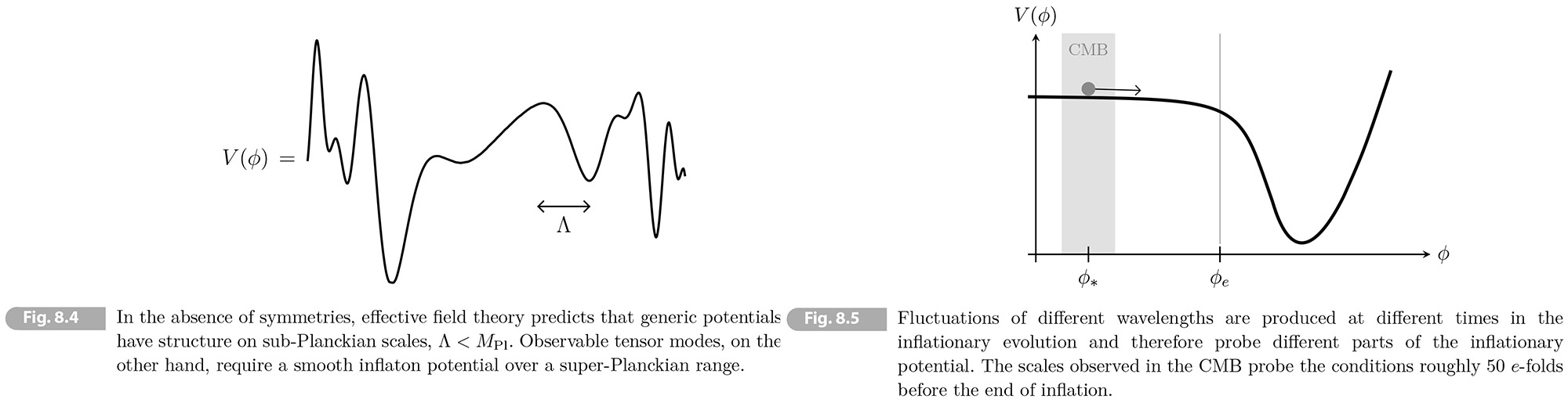
where 𝑐𝑛 are dimensionless Wilson coefficients that are typically of order one. We expect that the functional form of the potential will change when the field moves a distance of order 𝛬: in other orders, there is "structure" in the potential on scales of order 𝛬 (see Fig. 8.4). Even under the optimistic assumption that 𝛬 ≈ 𝑀𝑃𝑙, the potential (8.123) will not support large-field inflation unless one effectively finetunes the infinite set of Wilson coefficients 𝑐𝑛.
The leading idea foe implementing large-field inflation is to use a symmetry to suppress the dangerous higher-dimension contributions in (8.123). For example, an unbroken shift symmetry,
(8.124) 𝜙 ↦ 𝜙 + const,
forbids all non-derivative interactions, including the desirable parts of the inflaton potential, while a suitable weakly broken shift symmetry2 can give rise to a radiatively stable model of large-filed inflation. Whether such a shift symmetry can be UV-completed is a subtle and important question for a Planckian-scale theory like string theory. This is discussed in more detail in D. Baumann's book with L. McAllister [1] and explicit examples of large-field inflation in string theory were developed in [7, 8].
8.3.3 Slow-Roll Predictions
So far, we have expressed the inflatinary predictions in terms of the Hubble rate during inflation, evaluated at the time when the modes of interest exited the horizon. We would like to related this to the shape of the shape of the potential in slow-roll inflation. Using the relation between the Hubble and potential slow-roll parameters derived in (4.66), we can write the amplitude of the scalar spectrum (8.97) and its tilt (8.98) as
(8.125) 𝛢𝑠 = 1/24π2 1/𝜀𝑉, 𝑉*/𝑀𝑃𝑙4,
(8.126) 𝑛𝑠 - 1 = -6𝜀𝑉,* + 2𝜂𝑉,*,
where 𝜀𝑉 and 𝜂𝑉 were defined in (4.65). Similarly, the amplitude of the tensor spectrum (8.115) and its tilt (8.116) become
(8.127) 𝛢𝑡 = 2/3π2 𝑉*/𝑀𝑃𝑙4,
(8.128) 𝑛𝑡 = -2𝜀𝑉,*.
Observations near the reference scale 𝑘* then probe the shape of the inflaton potential around 𝜙* ≡ 𝜙(𝑡*), where 𝑡* is the moment of horizon crossing of the fluctuation with wavenumber 𝑘* (see Fig. 8.5). The largest observable fluctuations are probed in the CMB and exit the horizon at early times. Short-wavelength fluctuations exit the horizon later as the field has rolled further down its potential.
It is often useful to define the moment of horizon exit by the number of 𝑒-folds remaining until the end of inflation
(8.129) 𝑁* ≡ ∫𝜙𝑒𝜙* 𝐻/𝜙̇ d𝜙 ≈ ∫𝜙𝑒𝜙* 1/√(2𝜀𝑉) ∣d𝜙∣/𝑀𝑃𝑙,
where 𝜙𝑒 is the field value at which 𝜀𝑉 = 1. CMB observations probe a range of about 7 𝑒-folds centered around 𝑁* ~ 50 𝑒-folds before the end of inflation.
Case study: quadratic inflation
Let us illustrate the slow-roll predictions for 𝑚2𝜙2 inflation. In Chapter 4, we showed that the slow-roll parameters of this model are
(8.130) 𝜀𝑉(𝜙) = 𝜂𝑉(𝜙) = 2𝑀𝑃𝑙2/𝜙2,
and the number of 𝑒-folds before the end of inflation is
(8.131) 𝑁(𝜙) = 𝜙2/4𝑀𝑃𝑙2 - 1/2 ≈ 𝜙2/4𝑀𝑃𝑙2.
At the time when the fluctuation which eventually created the CMB anisotripoies crossed the horizon, we have
(8.132) 𝜀𝑉,* = 𝜂𝑉,* ≈ 1/𝑁* ≈ 0.01,
where the final equality is for a fiducial value of 𝑁* ≈ 50. The spectral tilt and the tensor-to-scalar ratio then are
(8.133) 𝑛𝑠 ≡ 1 - 6𝜀𝑉,* + 2𝜂𝑉,* = 1 -2/𝑁* ≈ 0.96,
(8.134) 𝑟 ≡ 16𝜀𝑉,* = 8/𝑁* ≈ 0.16.
As we will see in Section 8.4, the relatively large value of the tensor-to-scalar ratio is inconsistent with the data, so the model is ruled out. We can explore predictions of other slow-roll models in the problems in this chapter.
2 Note that to realize an approximate shift symmetry in the low-energy theory, it would suffice for the inflaton to have weak couplings 𝑔 ≪ 1 to all the degrees of freedom of the UV completion; the Wilson coefficients in (8.123) would then be suppressed by powers of 𝑔. Equivalently, the effective cufoff scale would become 𝑀𝑃𝑙/𝑔 ≫ 𝑀𝑃𝑙 and the coupling of the coupling of the inflaton to any additional degrees of freedom would be weaker than gravitational [6]. |
|
|