|
김관석
|
2024-12-03 17:49:50, 조회수 : 55 |
- Download #1 : BC_7c.jpg (998.6 KB), Download : 1

7.4.5 Summary of Results
Weinberg's semi-analytic solutions for Sachs-Wolfe and Doppler transfer functions are
(7.141) 𝐹*(𝑘) = 1/5 [𝑒-𝑘2/𝑘𝐷,*2𝑆(𝑘)/(1 + 𝑅*)1/4 cos[𝑘𝑟𝑠,* + 𝜃(𝑘)] - 3𝑅*𝛵(𝑘)],
(7.142) 𝐺*(𝑘) = -√3/5 𝑒-𝑘2/𝑘𝐷,*2𝑆(𝑘)/(1 + 𝑅*)3/4 sin[𝑘𝑟𝑠,* + 𝜃(𝑘)]
here the interpolation functions 𝑆(𝑘), 𝛵(𝑘) and 𝜃(𝑘) are defined in (7.116) and plotted in Fig. 7.13. Using the result of Exercise 7.3, the power spectrum can be written as
(7.143) 𝑙(𝑙 + 1)/2π 𝐶𝑙 = ∫∞1 d𝛽/𝛽2√(𝛽2 - 1) [𝐹*2(𝑙𝛽/𝜒*) + (𝛽2 - 1)/𝛽2 𝐺*2(𝑙𝛽/𝜒*)]∆𝓡2(𝑙𝛽/𝜒*),
The integral converges rapidly and accurate results are obtained with a relatively low cutoff at 𝛽 = 5 [Weinberg]. Since most of support is near 𝛽 = 1, the power spectrum is the sum of the two transfer functions, evaluated at 𝑘 ≈ 𝑙/𝜒* . The full spectrum must also include the ISW contribution and the cross correlations between the (I)SW and Doppler contributions.
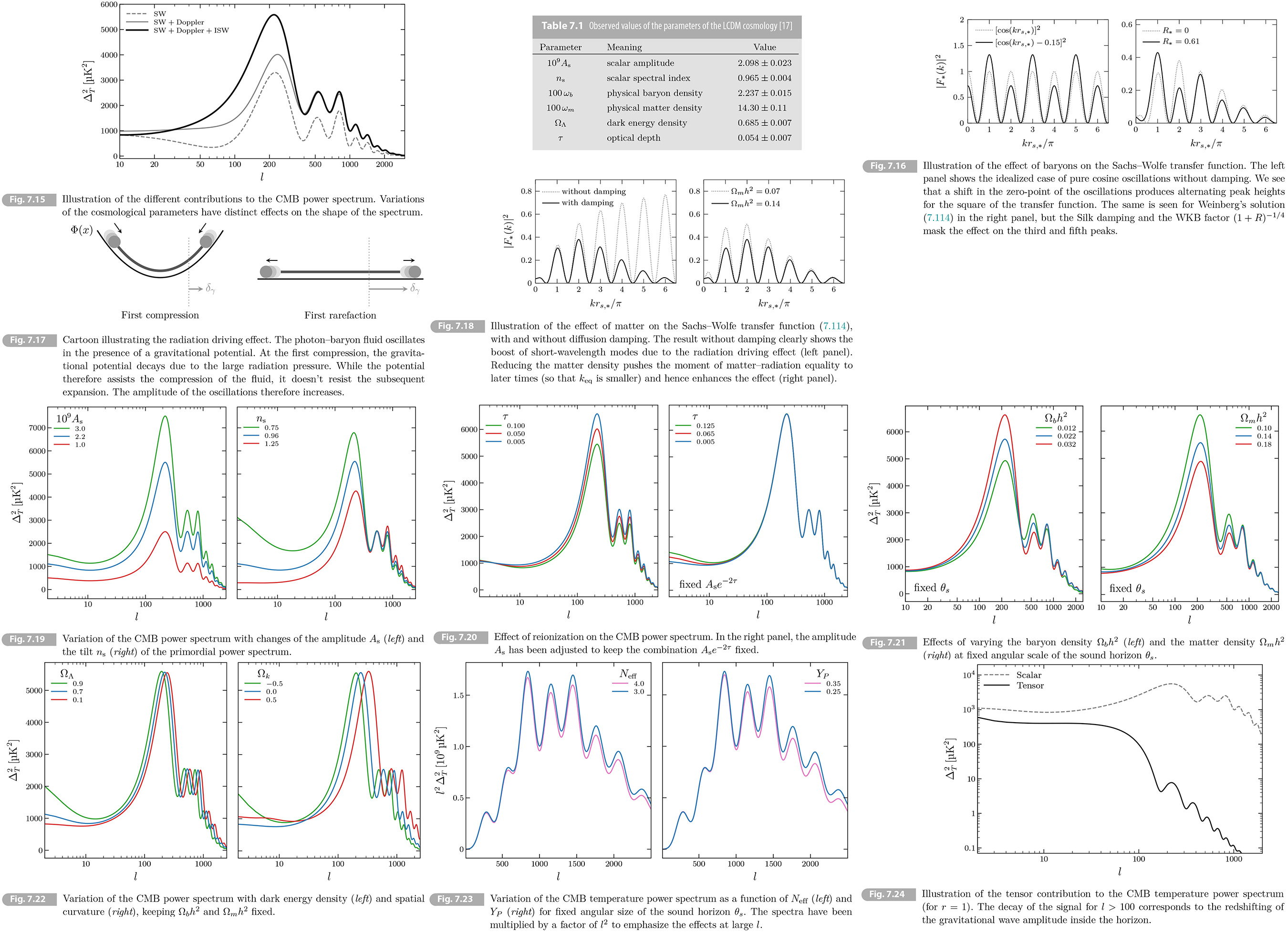
Fig. 7.15 shows the different contributions to the CMB power spectrum. We see that most of the shape of the spectrum comes from SW term, with the Doppler term slightly reducing the contrast between the peaks and troughs. The ISW effect has a significant effect on the height of the first peak.We will discuss how the shape of the spectrum depends on the cosmological parameters.
7.5 Understanding the Power Spectrum
The 𝛬CDM model is defined by six parameters, which are
{𝛢𝑠, 𝑛𝑠, 𝜔𝑏, 𝜔𝑚, 𝛺𝛬, 𝜏}
𝛢𝑠 and 𝑛𝑠 describe the spectrum of the initial curvature perturbations. The remaining four parameters determine the evolution of the fluctuations as well as their projection onto the sky. The physical baryon and mater densities, 𝜔𝑏 ≡ 𝛺𝑏𝘩2 and 𝜔𝑚 ≡ 𝛺𝑚𝘩2, where 𝘩 is the dimensionless Hubble constant. The fractional density in the cosmological constant is 𝛺𝛬. The photon density is fixed by the measured CMB temperature 𝛵0 = 2.725 K. Neutrinos are treated as massless, so that their density is fixed in terms of the photon density. A nonzero neutrino mass is easy to incorporate and can be constrained by its effect on the gravitationally lensed spectrum. The Hubble constant 𝐻0 (or 𝘩) is not a free parameter because we are assuming a flat universe, so that 𝘩 = √[𝜔𝑚/(1 - 𝛺𝛬)]. The final parameter 𝜏 is the integrated optical depth to recombination, [RE (3.87)] which is nonzero because the light of the first stars reionized the universe. The measured values of the base parameters of the 𝛬CDM cosmology are given in Table 7.1.
7.5.1 Peak Locations
The key characteristics of the CMB spectrum are the positions and heights of the acoustic peaks. The angular scale of the acoustic peaks is given by 𝜃𝑠 ≡ 𝑟𝑠,*/𝑑𝛢,*, where 𝑟𝑠,* is the sound horizon at decoupling and 𝑑𝛢,* is the comoving angular diameter distance to the last-scattering surface (see Section 2.2.3). In this chapter we assumed a flat universe where 𝑑𝛢,* = 𝜒*. The sound horizon depends on pre-recombination physics, so in 𝛬CDM model it is determined by 𝜔𝑏 and 𝜔𝑚 alone (for fixed radiation density). On the other hand the distance to last-scattering depends on the geometry (𝛺𝑘, 𝐻0 and the energy content (𝛺𝛬, 𝛺𝑚) after recombination. Breaking the degeneracy between pre- and post-recombination physics requires additional data set(e.g. BAO data or supernovae). [RE Wikipedia BAO]
7.5.2 Peak Heights
The peak heights are determined by four distinct effects:
1. Diffusion damping Recall that the diffusion length is roughly the geometric mean of the photon mean free path and the age of the universe at recombination. The former depends on the baryon density (𝜔𝑏), while the latter is a function of the total matter density (𝜔𝑚).
2. Early ISW effect As in Section 7.2.3 the residual radiation density at recombination lead to a time dependence in the potential, 𝛷ʹ ≠ 0, which affects the gravitational redshift of the CMB photons. Since 𝛷 is small on small scales, the main effect is on the first peak of the spectrum.8
3. Baryon loading Baryon add extra weight to the fluid which displaces the zeropoint of the acoustic oscillations. This "baryon loading" changes the relative heights of the odd and even peaks. The heights of alternating peaks are therefore a measure of the baryon density.
4. Radiation driving Changes in the relative amount of matter and radiation affect the peak heights through an effect called "radiation driving." Reducing the amount of matter increases the height of the first few peaks. Since the radiation density is fixed by the CMB temperature, this provides a way to measure the total matter density of the universe.
The last two effects deserve further explanation.
Baryon loading
Baryons contribute to both the initial and gravitational mass of the photon-baryon fluid, 𝑚eff ∝1 + 𝑅, but not to the pressure. Increasing the baryon density change the pressure and gravity in the evolution of the photon-baryon fluid.
One characteristic effect of this "baryon loading" is the shift of the zero-point of the oscillations, described by the -3𝑅𝛵(𝑘) term in (7.114). Since the CMB power spectrum depends on the square of the the transfer function, this shift of the zero-point leads to dfferences in the heights of alternating peaks (see Fig. 7.16). The effect is clearly seen in Weinberg's solution for SW transfer function, although the impact on the heights of the third and fifth peaks is masked by the damping of fluctuations.
The time dependence of the baryon-to-photon ratio 𝑅 affects the amplitude of the acoustic oscillation through the WKB factor (1 + 𝑅)-1/4 in (7.11). Consider the analogy with, in classic mechanics, the ratio of the energy 𝐸 = 1/2 𝑚eff𝜔2𝛢2 to the frequency 𝜔 of an oscillator is an adiabatic invariant. In our case, the evolution of 𝑅 induces a slow evolution of the sound speed and hence the oscillation frequency 𝜔 ∝ (1 + 𝑅-1/2. Combining this with 𝑚eff ∝ (1 + 𝑅), the constraint 𝑚eff𝜔𝛢2 = const leads to 𝛢 ∝ (1 + 𝑅)-1/4.
Radiation driving
As in Section 6.3.1, the gravitational potential decays when a mode enters the horizon during the radiation era. This leads to a boost the amplitude of the fluctuation captured by the transfer function 𝑆(𝑘) in (7.11.1). Intuitively, this can be understand as follows: the moment at which the potential starts to decay coincides with the compression of the photon-baryon fluid, since both begin at horizon crossing. The potential assists the first compression of the fluid through a near-resonant driving force, but doesn't resist the subsequent rarefaction of the fluid (see Fig. 7.17). That amplitude of the acoustic oscillations therefore increase. Additionally the time-dependent potential 𝛷(𝜂̄) induces a time dilation effect in the force term cf. (7.63), which increase the amplitude of the photon fluctuations. Heuristically an overdensity (with negative a 𝛷) induces a "stretching: of the space as in (7.13). As the potential decays the space "re-contracts" and the photons are blueshifted. The combination of the two effects boosts by a factor of about 5. The effect is clearly seen in Weinberg's solution for the SW transfer function, cf. Fig. 7.18.
Only modes that enters the sound horizon during radiation-dominated epoch experience this "radiation driving." We expect the amplitude of the peaks in the CMB to increase as we go from low multipoles to high ones, with the point of the transition depending of the relative amount of matter and radiation in the universe.
7.5.3 𝛬CDM Cosmology
WE are now ready to explain how the CMB spectrum depends on the base parameters of the 𝛬CDM model, {𝛢𝑠, 𝑛𝑠, 𝜔𝑏, 𝜔𝑚, 𝛺𝛬, 𝜏}.
Initial conditions
Our computation of the CMB spectrum assume a power law ansatz for the power spectrum of primordial curvature perturbations
(7.144) ∆𝑅2(𝑘) = 𝛢𝑠(𝑘/𝑘0))𝑛𝑠 - 1,
where 𝑘0 = 0.05 Mpc-1 is an arbitrary chosen pivot scale. Since the evolution is linear, it is easy to understand how changes in the amplitude 𝛢𝑠 and the tilt 𝑛𝑠 affect the observed spectrum. 𝛢𝑠s simply rescale the overall amplitude, while 𝑛𝑠s changes the relative amount of power on large and small scales (see Fig. 7.19).
One of the most remarkable discoveries from CMB is that the primordial spectrum is close to scale invariant, but not exactly: 𝑛𝑠 = 0.965 ± 0.004 [17]. In Chapter 8 we will see this deviation is a prediction of inflation, where it arises from slow decay of the inflationary energy density. The measurement of the parameter 𝑛𝑠 is our first measurement of the dynamics during inflation. We will study more about this in the next chapter.
Reionization
There is an effect, not yet mentioned, that also affects the overall amplitude. The ultraviolet light from the first stars reionized the universe, so that the CMB photons have a small probability to scatter off the free electrons in the late universe. To quantify this, consider a photon on a direction 𝐧̂ , with temperature 𝛵(𝐧̂) = 𝛵̄[1 + 𝛩(𝐧̂)]. The probability of no scattering to occur is 𝑒-𝑟, while the probability of rescattering is 1 - 𝑒-𝑟. The temperature of the rescattered photons will be the temperature 𝛵̄ of the equilibrated ionized regions. The observed temperature today is
(7.145) 𝛵0(𝐧̂) = 𝛵0̄[1 + 𝛩(𝐧̂)]𝑒-𝑟 + 𝛵0̄(1 - 𝑒-𝑟) = 𝛵0̄[1 + 𝛩(𝐧̂)𝑒-𝑟].
We see that the observed anisotropies are suppressed by a factor of 𝑒-𝑟 and the power spectrum becomes
(7.146) 𝐶𝑙 → 𝐶𝑙𝑒-2𝑟.
The effect only occurs on scales that are smaller than the horizon at reionization corresponding to multipoles 𝑙 > 0. Since the power spectrum is uniformly reduced by a factor of 𝑒-2𝑟, the impact of reionization is degenerate with a change of amplitude 𝛢𝑠; observation only constrain the combination 𝛢𝑠𝑒-2𝑟 (see Fig. 7.20). To break this degeneracy requires an independent measurement of the optical depth 𝜏. This is provided by CMB polarization (see Section 7.6).
Baryons
A change in the baryon density 𝜔𝑏 has three main effects:
1. It changes the sound speed and hence lead to a different sound horizon at recombination,
(7.147) 𝑟𝑠,* = ∫𝑎*0 (d ln 𝑎)/𝑎𝐻 𝑐𝑠(𝑎).
Associated with the change in 𝑟𝑠,* is a change in angular scale of the sound horizon 𝜃𝑠 = 𝑟𝑠,*/𝜒*, where s the comoving distance to the last-scattering surface
(7.148) 𝜒* = ∫1𝑎* (d ln 𝑎)/𝑎𝐻.
The value of 𝜃𝑠 determines the peak locations of the CMB spectrum.
2. It changes the zero-point of the acoustic oscillations, enhancing the difference in the heights of odd and even peaks in the spectrum (see Section 7.5.2).
3. It affects the damping of the fluctuations. Reducing the baryon density reduces the tight coupling between the photons and baryons and hence increases the damping effect.
The effect on the peak locations is degenerate with other parameters (such as the dark energy density 𝛺𝛬) that change the distance to last-scattering 𝜒* and hence the observed angular scale 𝜃𝑠. In the left panel of Fig. 21. the spectrum for some 𝜔𝑏 but fixed 𝜃𝑠 was therefore plotted. This removes the effect on the peak locations and highlights the effect on the peak amplitudes. We see that increasing 𝜔𝑏 raises the first peak and suppresses the second peak, as expected the discussion on baryon loading. Fr the higher peaks the Silk damping and the WKB factor (1 + R)-1/4 mask the effect. Looking closely at the spectrum for 𝑙 > 1000, we also see the enhanced damping of the fluctuations for reduced baryon density.
The observation of the CMB lead to 𝜔𝑏 = 0.02237 ± 0.00015 or 𝛺𝑏 = 0.0493 ± 0.0006 [17]. As in Section 3.2.4, this value is consistent with the value required by BBN.
Dark Matter
A change in 𝜔𝑚 has four main effects:
1. It changes the Sound horizon t recombination through a change in the evolution of the Hubble rate cf (7.147). It also affects 𝜒* The combination of the two effects determines the angular scale of 𝜃𝑠 and hence the peak locations.
2. It shifts the time of matter-radiation equality. Reducing the matter density shifts the moment of equality to a later time which enhances the radiation driving effect described in Section 7.5.2 and hence increases the peak heights.
3. It determines the early ISW effect by changing the relative amount matter and radiation at the time of recombination. Reducing the matter density increases the early ISW effect, which leads to a boost in the height of the first peak.
4. It affects the diffusion scale by changing the time to recombination.
In the right panel of Fig. 7.21, The CMB spectrum for different value of 𝜔𝑚. As expected, reducing the matter density leads to a boost in the amplitudes of the few peaks. The effect saturates for lower* peaks
which aren't t affected by changes in the matter density. [correction*: higher in original text]
The observations give 𝜔𝑚 = 0.1430 ± 0.0011 or 𝛺𝑚 = 0.3153 ± 0.0073 [17]. Comparing this to the measurement of the baryon density, we conclude that the universe must have non-baryonic dark matter. The measured amount of the dark matter is consistent with the requirement from formation discussed in Chapter 5 and 6.
Dark Energy
Changing the dark energy density 𝛺𝛬 affects the CMB spectrum mainly through its effect on the distance to the last-scattering surface. The latter depends on the Hubble rate after recombination, which in a flat universe is
(7.149) 𝛨2(𝑎) = 𝛨02 (𝛺𝑚𝑎-3 + 𝛺𝛬).
Since the matter density is constrained by its effect o the peak heights, this allows us to measure the dark energy density. Increasing 𝛺𝛬 at fixed 𝛺𝑚𝘩2 increases the Hubble rate and decreases the distance to last-scattering, so that the peaks move to larger angular scale (lower 𝑙). This is what is seen in Fig. 7.22. Since dark energy affects the CMB mostly through its effect on the distance to last-scattering, it is degenerate with any other parameter that also changes its distance, such as spatial curvature. Breaking this geometric degeneracy requires either external data data set or a measurement of CMB lensing. Combing measurements of the CMB and BAO gives 𝛺𝛬 = 0.685 ± 0.007 [17].
As we can see from Fig. 7.22, increasing the amount of dark energy also leads to an increase in the power on large scales (low 𝑙). This arises from late ISW effect, The onset of dark energy induces a decay of the gravitational potential, which reduces the net gravitational redshift in traversing the large-scale time-varying gravitational potentials and hence increases the large-scale CMB temperature fluctuations.
Curvature
We assumed a spatially flat universe until now. We may ask how the CMB can test if the universe is really flat. Physical scales on the last-scattering surface are related to the observed angular scales by the (comoving) angular diameter distance 𝑑𝛢,*. For small deviation from a flat universe, we have
(7.150) 𝑑𝛢,* = { 𝑅0 sin(𝜒*/𝑅0) ≈ 𝜒*(1 - 𝜒*2/6𝑅02) (positively curved); 𝑅0 sinh(𝜒*/𝑅0) ≈ 𝜒*(1 + 𝜒*2/6𝑅02) (negatively curved).
We see that the angular diameter distance increases for a negatively curved universe. The peaks in the CMB spectrum move to smaller scale (larger multipoles) and vice versa. This is what is seen in Fig. 7.22. (Recall 𝛺𝑘 < 0 for a positvely curved universe.) The figure also illustrates on the low-𝑙 spectrum the significant effect through its impact on the late ISW effect.
Hubble constant
Our parameterization of 𝛬CDM model in (7.144) did not include Hubble constant. Assuming a flat universe the Friedmann equation relates the Hubble constant to 𝛺𝑚 and 𝛺𝛬. We could also have used Hubble constant as a free parameter and made the dark energy density a derived parameter. In that case, the Hubble rate in (7.149) would be written as
(7.151) 𝐻2(𝑎) ∝ (𝜔𝑚𝑎-3 + 𝘩2 - 𝜔𝑚). [verification needed]
Constraining 𝜔𝑚 through its effect on the peak heights (and/or external data sets) then allows the CMB to measure the Hubble constant 𝘩 (𝐻0). These observation finds 𝘩 = 0.674 ± 0.005 [17]. Interestingly, there is somewhat in tension with local measurements using supernovae, which gives 𝘩 = 0.730 ± 0.010 [18]. This so called "Hubble tension" remain an important open problem of the 𝛬CDM model.
7.5.4 Beyond 𝛬CDM
As extensions beyond the 𝛬CDM cosmology, we will discuss the two well-motivated examples: extra relativistic species and tensor modes.
Extra relativistic species
In the 𝛬CDM model, the radiation density is fixed in therms of the CMB temperature. However extra ligh species or non-standard neutrino properties can lead to extra radiation density.
The total energy density in relativistic species is often defined as [RE (3.66)]
(7.152) 𝜌𝑟 = [1 + 7/8 (4/11)4/3 𝑁eff]𝜌𝛾,
where 𝜌𝛾 is the energy density of photons. 𝑁eff is referred to as "effective number of neutrinos," although there may be contributions to it that have nothing to do with neutrinos. The Standard Model predicts 𝑁eff = 3.046 and the current constraint from the Planck satellite is 𝑁eff = 2.99±0.17 [17]. Deviations from the standard value may arise if the neutrinos have non-standard properties or if new physics at high energies leads to additional weakly coupled light species (see Problem 3.5).
The main effect of adding extra radiation to the early universe is to increase the damping of the CMB spectrum (see Fig. 7.23. Increasing 𝑁eff increases 𝐻*, the expansion rate at recombination. This would change both the damping scale 𝜃𝐷 and the acoustic scale 𝜃𝑠, with the ratio scaling as [RE (7.54-55) (7.147)]
(7.153) 𝜃𝐷/𝜃𝑠 = 1/𝑟𝑠,*𝑘𝐷 ∝ 1/𝐻*-1𝐻*1/2 = 𝐻*1/2. [verification needed]
Since 𝜃𝑠 is measured very accurately by the peak locations, we need to keep it fixed. His can be done, for example, by simultaneously increasing the Hubble constant 𝐻0. Increasing 𝑁eff (and hence 𝐻*) at fixed 𝜃𝑠 then implies larger 𝜃𝐷, so that the damping kicks in at larger scales, reducing the power in the damping tail (see Fig. &.23). By accurately measuring the small-scale CMB anisotropies observations can put a constraint on the number of relativistic species at recombination.
The main limiting factor in these measurements is a degeneracy with the primordial helium fraction 𝑌𝑃 ≡ 4𝑛He/𝑛𝑏. [RE (3.115)(3.141)] At fixed 𝜔𝑏, increasing 𝑌𝑃 decreases the number density of free electrons, which increases the diffusion length and hence reduces the power in the damping tail. 𝑌𝑃 and 𝑁eff are anti-correlated.[verification needed] This degeneracy is broken by the phase shift induced by free-streaming relativistic species [13, 14].
As shown in Problem 3.5 light particles that decoupled before the QCD phase transition contribute at the percent level to the radiation density of the universe. Although such a signal is an order of magnitude smaller than the sensitivity of current CMB observations, it is within reach of the next generation of CMB experiments [19].
Gravitational waves
In Problem 7.6 we will explore the impact of tensor metric fluctuations, 𝛿𝑔𝑖𝑗 = 𝑎2𝘩𝑖𝑗, on the CMB temperature fluctuations. [RE (6.208)] The presence of these gravitational waves creates temperature anisotropies at last-scattering, as can be determined from geodesic equation for photons. In Problem 7.6 we will find the line-of -sight solution is
(7.154) 𝛳(𝑡)(𝐧̂) = -1/2 ∫𝜂0𝜂* d𝜂 𝘩𝑖𝑗ʹ𝜂̂𝑖𝜂̂𝑗.
Moreover we will show that the tensor-induced power spectrum is
(7.155) 𝐶𝑙(𝑡) = 4π ∫ d ln 𝑘 ∣𝛳𝑙(𝑡)(𝑘)∣2 ∆𝘩2(𝑘),
where ∆𝘩2(𝑘) is the primordial power spectrum of the tensor mode (as defined in Section 6.5). In problem 7.6, we will derive an explicit form for tensor function 𝛳𝑙(𝑡)(𝑘). A scale-invariant tensor spectrum ∆𝘩2(𝑘) ≈ const, lead to 𝑙(𝑙 + 1)𝐶𝑙(𝑡) ≈ const on large scales. On small scales we expect the signal to be suppressed since the amplitude of the gravitational waves decays inside the horizon. This is confirmed by the numerical result in Fig. 7.24.
The measurement of the large-scale CMB temperature anisotropy spectrum constrains the tensor amplitude to 𝑟 < 0.1 [170, where 𝑟 ≡ ∆𝘩2(𝑘0)/∆𝑅2(𝑘0) is the tensor-to-scalar ratio. Stronger constrains on 𝑟 require the measurement of CMB polarization, especially its B-mode type.
8 Another important effect is that the early ISW effect continues to increase the poer even after decoupling. This is the reason that the first peak not only taller, but also fatter, extending to lower multipoles, see Fig. 7.15. |
|
|