|
김관석
|
2024-09-06 13:05:31, 조회수 : 117 |
- Download #1 : BC_3a.jpg (203.7 KB), Download : 1

3 The Hot Big Bang
The early universe was hot and dense. Above 104 K[≈ 1 eV], stable atoms didn't exist because the average energy of particles was larger than the binding energies of atoms. The universe was therefore a plasma of free electrons and nuclei, with high-energy photons scattering between them. Above 109 K, the nuclei had dissolved into their constituent protons and neutrons. The rate of interactions in the primordial plasma was very high and the universe was in a state of thermal equilibrium. The equilibrium state provides the initial conditions for the hot Big Bang. It is a very simple state in which the abundance of all the particle species are by determined by the temperature of the universe.
As the temperature decreased, these particles dropped out of the thermal equilibrium and decoupled from the thermal bath. Non-equilibrium dynamics is required for massive particles to maintain significant abundances. Deviation from equilibrium are also crucial for understanding CMB and the formation of the light chemical elements
Some key events in the thermal history of the universe are listed in Table 3.1. Our story in this chapter will begin one second after the Big Bang. There were mostly free electrons (𝑒-), positrons (𝑒+), photons (𝛾) and neutrinos (𝜈). A small amount were protons (𝑝+) and neutrons (𝑛).1 The photons were trapped the large density of free electrons.2 Neutrinos interacted with the rest of the primordial plasma through the weak nuclear interaction. The rate of these interaction soon dropped below cosmic neutrino background (C𝜈B), which still fills the universe today, but has such low energy that it is hard to detect directly. Electrons and positrons annihilated into photons shortly after neutrino decoupling. The energy of them got transferred to the photons, but not to the neutrinos. This resulted in a slight increase in the photon temperature relative to the neutrino temperature. Around three minutes later, Big Bang nucleosynthesis (BBN) took place, which fused protons and neutrons into light elements-mostly deuterium, helium and lithium. The next event, recombination occurred 370 000 years after the Big Bang. At this moment, the temperature became low enough for hydrogen atoms to form through the reaction 𝑒- + 𝑝+ → 𝐻 + 𝛾. Before recombination, the strongest coupling between the photons and the rest of the plasma was through Thomson scattering, 𝑒- + 𝛾. The sharp drop in the free electron density after recombination meant that this process became very inefficient and the photons decoupled. They have since streamed freely through the universe and are today observed as the cosmic microwave background (CMB).
It is remarkable that this story of the hot Big Bang can now be told as a scientific fact.
* * *Let us start with so-called natural units, where the speed of light and the reduced Planck constant are set to unity
(3.1) 𝑐 = ℏ ≡ 1.
In these units, length and time have the units, and are inverse of mass and energy. We will also introduce the reduced Planck mass
(3.2) 𝑀𝑃𝑙 = √(ℏ𝑐/8π𝐺) = 2.4 × 10¹⁸ 𝐺𝑒𝑉,
so that the Friedmann equation for a flat universe reads 𝐻2 = 𝜌/3𝑀𝑃𝑙2. Finally, we will often set Boltzmann's constant equal to unity, 𝜅𝛣 ≡ 1, so that temperature has units of energy. Useful conversions are
(3.3) 𝑚𝑝 = 1.60 × 10¹⁰ J = 1.16 × 10¹³ K = 1.78 × 10⁻²⁷ kg = (1.97 × 10⁻¹⁶ J)-1 = (6.65 × 10⁻²⁵ s)-1,
where 𝑚𝑝 is the proton mass. For more about the concept of natural units, refer to the beginning of Appendix C.
3.1 Thermal Equilibrium
The blackbody spectrum of the CMB is strong observational evidence that the early universe was in a state of thermal equilibrium.3 Moreover, on theoretical grounds, we expect the interactions of the Standard Model to have established thermal equilibrium at temperature above 100 GeV. In this section this initial state of the hot Big Bang and its subsequent evolution using the methods of thermodynamics and statistical mechanics, suitably generalized to apply to an expanding universe.
3.1.1 Some Statistical Mechanics
The early universe was a hot gas of weakly interacting particles. We will use a coarse-grained description of the gas using the principles of statistical mechanics. So we will characterize the properties of gas statistically. A lightning introduction to the relevant concepts of statistical mechanics and equilibrium thermodynamics will be given, if necessary, refer to some textbook on the subject.
Distribution functions
A key concept in statistical mechanics is the probability that a particle chose at random has a momentum 𝐩. In general, the probability function 𝑓(𝐩,𝑡) can be very complicate.4 However, if we wait long enough (relative to the typical interaction timescale), then the system will reach equilibrium and is characterized by a time-independent function. At this time, the gas has reached a state of maximum entropy in which the distribution function is given by either the Fermi-Dirac distribution (for fermions) or the Bose-Einstein distribution (for bosons)
(3.4) 𝑓(𝑝,𝛵) = 1/[𝑒(𝐸(𝑝) - 𝜇)/𝛵 ± 1],
where the + sign for fermions and - sign for bosons. For a derivation of these functions refer to any textbook on statistical mechanics. The function in (3.4) has two parameters: temperature, 𝛵, and chemical potential, 𝜇. The latter describes the response of a system to a change in the particle number and can be positive or negative (see Section 3.1.5). The chemical potential may be temperature dependent, and since the temperature changes in an expanding universe, even the equilibrium distribution functions depend implicitly on time.
Density of states
To relate this microscopic description of the gas to its macroscopic properties, we must sum over all possible momentum states of the particles weighted by their probabilities. For example, the number density of particles in the gas is
(3.5) 𝑛 = ∑𝐩 𝑓(𝑝,𝛵).
To define this sum over state as an integral over the continuous variable 𝐩, requires the density of states. It is easiest to derive this density of states by considering the gas as a quantum system. In quantum mechanics, the momentum eigenstates of a particle in a box of side 𝐿 have a discrete spectrum. Solving the Schrödinger equation with periodic boundary conditions gives
(3.6) 𝐩 = 𝘩/𝐿 (𝑟1𝐱 + 𝑟2𝐲 + 𝑟3𝐳),
where 𝑟𝑖 = 0, ±1, ±2, ... and 𝘩 = 4.14 × 10⁻¹⁵ eVs is Planck's constant. In momentum space, the states of particle are therefore represented by a discrete set of pints, The density states in momentum space {𝐩} then 𝐿3/𝘩3 = 𝑉/𝘩3, and the states density in phase space {𝐱, 𝐩} is 1/𝘩3, If the particle has 𝑔 internal degrees of freedom (e.g. due to the intrinsic spin of elementary particles), then the density of states becomes
(3.7) 𝑔/𝘩3 = 𝑔/(2π)3,
where we have used natural units with ℏ = 𝘩/((2π) ≡ 1.
Densities and pressure
Weighting each state by its probability distribution, and integrating over momentum, we obtain the number density particles
(3.8) 𝑛(𝛵) = 𝑔/(2π)3 ∫ 𝑑3𝑝 𝑓(𝑝,𝛵). [Wikipedia Multiple integral]
The energy density and pressure of the gas are then given by
(3.9) 𝜌(𝛵) = 𝑔/(2π)3 ∫ 𝑑3𝑝 𝑓(𝑝,𝛵) 𝐸(𝑝),
(3.10) 𝜌(𝛵) = 𝑔/(2π)3 ∫ 𝑑3𝑝 𝑓(𝑝,𝛵) 𝑝2/3𝐸(𝑝),
where 𝐸(𝑝) = √(𝑚2 + 𝑝2), [RE Wikipedia Energy–momentum relation] if we can ignore the interaction energies between the particles.5. The origin of the factor in the pressure require more explanation. The volume swept out in unit time is ∣𝑣𝑥∣𝑑𝛢 = ∣𝑝𝑥∣2𝑑𝛢/𝐸(𝑝) which for an isotropic distribution in three direction is 𝑝2/3𝐸(𝑝). *[corrected in simpler way by myself]
Each particle species 𝑖 (with possibly distinct 𝑚𝑖, 𝜇𝑖, 𝛵𝑖) has its own distribution function 𝑓𝑖 and hence its own densities and pressure, 𝑛𝑖, 𝜌𝑖, 𝑃𝑖. Species that are in thermal equilibrium share a common temperature, 𝛵𝑖 = 𝛵. Their densities and pressures can then only differ because of difference in their masses and chemical potentials.
At early times, the chemical potentials of all particles are much smaller than the temperature, ∣𝜇𝑖∣ ≪ 𝛵, and can be neglected. For electrons and protons this is provable fact, for photons ii holds by definition and for neutrinos it sis likely true, but not proven.
3.1.2 The Primordial Plasma
We will relate the densities and pressure of the different species in the different species in the primordial plasma to the overall temperature of the universe. Setting the chemical potential to zero, we get
(3.11) 𝑛 = 𝑔/2π2 ∫0∞ 𝑑𝑝 𝑝2/[exp{√(𝑝2 + 𝑚2)/𝛵} ± 1],
(3.12) 𝜌 = 𝑔/2π2 ∫0∞ 𝑑𝑝 𝑝2√(𝑝2 + 𝑚2)/[exp{√(𝑝2 + 𝑚2)/𝛵} ± 1].
Defining the dimensionless variables 𝑥 ≡ 𝑚/𝛵 and 𝜉 ≡ 𝑝/𝛵, this can be written as
(3.13) 𝑛 = 𝑔/2π2 𝛵3 𝐼±(𝑥), 𝐼±(𝑥) ≡ ∫0∞ 𝑑𝜉 𝜉2/[exp√(𝜉2 + 𝑥2) ± 1],
(3.14) 𝜌 = 𝑔/2π2 𝛵3 𝐽±(𝑥), 𝐽±(𝑥) ≡ ∫0∞ 𝑑𝜉 𝜉2√(𝜉2 + 𝑥2)/[exp√(𝜉2 + 𝑥2) ± 1].
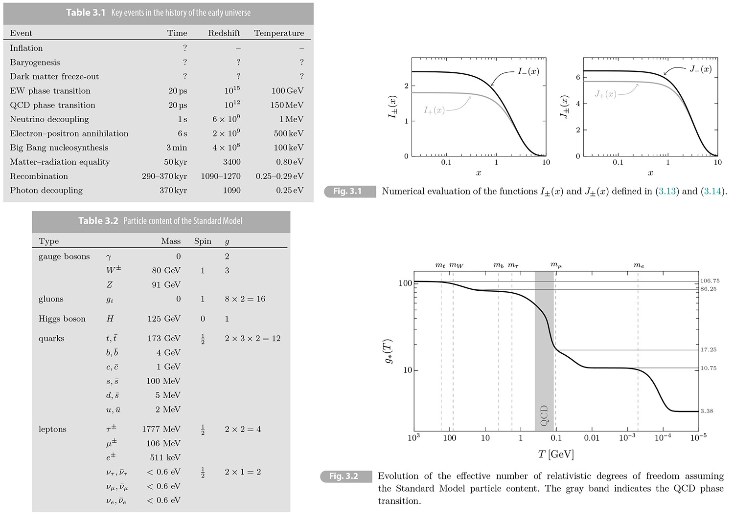
In general, the functions 𝐼±(𝑥) and 𝐽±(𝑥) have to be elevated numerically (see Fig. 3.1), but in the relativistic and non-relativistic limits, we can determine them analytically.
Relativistic limit
At temperatures much larger than the particle mass, we can take limit 𝑥[≡ 𝑚/𝛵] → 0 and the integral in (3.13) reduces to
(3.15) 𝐼±(0) = ∫0∞ 𝑑𝜉 𝜉2/𝑒𝜉 ± 1.
(3.16) 𝐼+(0) = 3/2 𝜁(3), 𝐼_(0) = 2 𝜁(3).
where we use Riemann zeta function 𝜁(3) = 1 + 1/23 + 1/33 + 1/43 + ∙ ∙ ∙ ≈ 1.20205
(3.17) 𝐼+(0)/𝐼_(0)= [3/2 𝜁(3)]/[2 𝜁(3)] = 3/4 ⇒ 𝐼+(0) = 3/4 𝐼_(0).
Substituting (3.17) into (3.13), we get
(3.18) 𝑛 = 𝜁(3)/π2 𝑔 𝛵3 { 1 bosons, 3/4 fermions.
A similar computation for energy density gives
(3.19) 𝐽±(0) = ∫0∞ 𝑑𝜉 𝜉3/𝑒𝜉 ± 1.
(3.20) 𝐽+(0) = 7/120 π4, 𝐽_(0) = 1/5 π4.
(3.21) 𝐽+(0)/𝐽_(0) = [7/120 π4]/[1/5 π4] = 7/8 ⇒ 𝐼+(0) = 7/8 𝐼_(0).
where we can use that 𝜁(4) = π4/90.
(3.22) 𝜌 = π2/30 𝑔 𝛵4 { 1 bosons, 7/8 fermions.
Exercise 3.1 Show that 𝐽_(0) = 6𝜁(4) and 𝐽+(0) = 7/8 𝐽_(0).
[Solution] 𝐽_(0) = 7/120 π4/𝜁(4) = (1/15 π4)/(π4/90) = 6𝜁(4) and refer to (3.21). ▮
Using the observed temperature of the CMB, 𝛵0 ≈ 2.73 𝐾, we find that the number density and energy density of photon today are
(3.24) 𝑛𝛾,0 = 2𝜁(3)/π2 𝛵03 ≈ 411 photons cm-3. [Wikipedia Cosmic microwave background, Photon gas]
(3.25) 𝜌𝛾,0 = π2/15 𝛵04 ≈ 4.17× 10⁻¹⁴ J cm-3. [verification. needed]
In terms of the critical density, the photon energy density is then found in the 𝛺𝛾𝘩2 ≈ 0.26 eV m-3. [verification. needed]
Finally, taking 𝑝 = 𝐸 in (3.10), we get
(3.26) 𝑃 = 1/3 𝜌,
as expected for a gas of relativistic particles ("radiation').
Non-relativistic limit
At temperature below the particle mass, we take the limit 𝑥 ≫ 1 and the integral in (3.13) in the same for bosons and fermions
(3.27) 𝐼±(𝑥) ≈ ∫0∞ 𝑑𝜉/[𝑒√(𝜉2 + 𝑥2)].
Most of contribution to the integral comes from 𝜉 ≪ 𝑥 [𝑥 ≡ 𝑚/𝛵, mass] and we can Taylor expand the square root, [√(𝜉2 + 𝑥2 ≈ 𝑥 + 𝜉2/2𝑥 at 𝜉 = 0], when in the exponential to the lowest order in 𝜉,
(3.28) 𝐼±(𝑥) ≈ ∫0∞ 𝑑𝜉 𝜉2/[𝑒{𝑥 + 𝜉2/(2𝑥)}]
Performing the Gaussian integral, we get [Wikipedia Gaussian integral : ∫-∞∞ 𝑒-𝑥2 = √ π.]
(3.29) 𝐼±(𝑥) ≈ √(π/2) 𝑥3/2 𝑒-𝑥,
and, using (3.16), we find
(3.30) 𝐼±(𝑥)/𝐼±(0) ≈ 0.5 𝑥3/2 𝑒-𝑥 ≪ 1.
As expected massive particles are exponentially rare at low temperatures.
Substituting (3.29) into (3.13), we can write the density of the non-relativistic gas as a function of the temperature
(3.31) 𝑛 = 𝑔 (𝑚𝛵/2π)3/2 𝑒-𝑚/𝛵
To determine the energy density in the non-relativistic limit, we can write 𝐸(𝑝) = √(𝑚2 + 𝑝2) ≈ 𝑚 + 𝑝2/2𝑚, [𝐸(𝑝) = √(𝑚2𝑐4 + 𝑝2𝑐2), 𝑐 ≡ 1.] We then find
(3.32) 𝜌 ≈ 𝑚𝑛 + 3/2 𝑛𝛵.
where the leading term is simply equal to the mass density.
Finally, from (3.10), it is easy to show that the pressure of a non-relativistic gas of particles is [verification. needed]
(3.33) 𝑃 = 𝑛𝛵,
which is nothing but the ideal gas law, 𝑃𝑉 = 𝑁𝑘𝐵𝛵 (for 𝑘𝐵 = 1). Since 𝛵 ≪ 𝑚, we have 𝑃 ≪ 𝜌, so that the gas acts like a pressureless fluid ("matter").
Exercise 3.2 Derive (3.32) and (3.33).
[Solution] We take the limit 𝑥 ≫ 1 and the integral in (3.13) in the same for bosons and fermions [𝑥 ≡ 𝑚/𝛵 and 𝜉 ≡ 𝑝/𝛵]
(a) 𝑛 = 𝑔/2π2 𝛵3 𝐼±(𝑥), 𝐼±(𝑥) ≡ ∫0∞ 𝑑𝜉 𝜉2/[exp√(𝜉2 + 𝑥2)] ≈ √(π/2) 𝑥3/2 𝑒-1
(b) 𝜌 = 𝑔/2π2 𝛵4 𝐽±(𝑥), 𝐽±(𝑥) ≡ ∫0∞ 𝑑𝜉 𝜉2√(𝜉2 + 𝑥2)/[exp√(𝜉2 + 𝑥2)].
Since in the non-relativistic limit, we can write 𝐸(𝑝) = √(𝑚2 + 𝑝2) ≈ 𝑚 + 𝑝2/2𝑚
(c) 𝜌 = 𝑔/2π2 𝛵4 𝐽±(𝑥), 𝐽±(𝑥) ≡ ∫0∞ 𝑑𝜉 𝜉2(𝑥 + 𝜉2/2𝑥)/[exp√(𝜉2 + 𝑥2) = 𝑥 𝐼±(𝑥) + 1/2𝑥 ∫0∞ 𝑑𝜉 𝜉4/[exp√(𝜉2 + 𝑥2)]
≈ ∫0∞ 𝑑𝜉 𝜉4/[𝑒{𝑥 + 𝜉2/(2𝑥)}] = 𝑥 𝐼±(𝑥) + 1/2𝑥 [3√(π/2) 𝑥3/2 𝑒-1] = 𝑥 𝐼±(𝑥) + 3/2 𝐼±(𝑥) ⇒ 𝜌 ≈ 𝑚 𝑛 + 3/2 𝑛 𝛵. ▮
By comparing the relativistic limit (𝛵 ≫ 𝑚) and the non-relativistic limit (𝛵 ≪ 𝑚), we see that the number density, energy density, and pressure of a particle species fall exponentially (are "Boltzmann suppressed") as the temperature drops below the mass of the particles. This can be interpreted as the annihilation of particles and antiparticles. At higher energies these annihilations also occurs, but they are balanced by by particle-antiparticle pair production. At low temperatures, the thermal energies of the particles aren't sufficient for pair production.
Relativistic species
The early universe was a collection of different species and the total density 𝜌 is the sum over all contributions
(3.34) 𝜌 = ∑𝑖 𝑔𝑖/2π2 𝛵𝑖4 𝐽±(𝑥𝑖),
where the different species can have different temperatures, 𝛵𝑖. For this complication is only relevant for neutrinos after electron-positron annihilation (see Section 3.1.4 to write ). It is common to write density in terms of the "temperature of the universe" 𝛵 (typically chosen to be photon temperature 𝛵𝛾),
(3.35) 𝜌 = π2/30 𝑔*(𝛵) 𝛵4,
where 𝑔* is defined as the "effective number of relativistic degree of freedom" at 𝛵, so
(3.36) 𝑔*(𝛵) ≡ ∑𝑖 𝑔𝑖 (𝛵𝑖/𝛵)4 𝐽±(𝑥𝑖)/ 𝐽_(0).
Since the energy density of relativistic species is much greater than that of non-relativistic species, it often suffices to include only the relativistic species in (3.36). Moreover, for 𝛵𝑖 ≫ 𝑚𝑖, we have 𝐽±(𝑥𝑖 ≪ 1) ≈ const and (3.36) reduces to
(3.37) 𝑔*(𝛵) ≡ ∑𝑖=𝑏𝑜 𝑔𝑖 (𝛵𝑖/𝛵)4 + 7/8 ∑𝑖=𝑓𝑒 𝑔𝑖 (𝛵𝑖/𝛵)4.
When all particles are in equilibrium at a common temperature 𝛵, determining 𝑔*(𝛵) is then simply a counting exercise.
Learning to count
At early times, 𝛵 ≳ 100 GeV, all particles of the Standard Model were relativistic (see Table 3.2. To determine the corresponding value of 𝑔*, we need to sum over the internal degree of freedom of each particle species.
Let us start with gauge bosons. Photons have 𝑔𝛾 = 2 corresponding to two polarizations transverse to the direction of propagation. In total massive boson of spin 𝑠 has 𝑔 = 2𝑠 + 1 polarization states. For the massive spin-1 gauge bosons, we have 𝑔𝑤±, 𝑧 = 3 and hence a total 3 × 3 = 9 internal degrees of freedom. Gluon are massless and therefore contribute 𝑔𝑔 = 2 and there are 8 of them, corresponding to the 8 generators of the group 𝑆𝑈(3),, so we get 8 × 2 = 16.
Next, among fermions the charged leptons (𝑒±, 𝜇±, 𝜏± particles) are spin-1/2 particles and therefore two spin states each. Including a factor of 2 for antiparticles, we have 3 × 2 × 2 = 12. Similarly, each quark contributes two spin states. There are 6 favors of quark (𝑡, 𝑏, 𝑐, 𝑠, 𝑑, 𝑢) and each comes in 3 different colors. Including a factor of 2 for antiparticles, we then have 6 × 2 × 3 × 2 = 72. Lastly, we must talk about neutrinos. Neutrinos are massive spin-1/2 and they only contribute 1 internal degree of freedom.
An aside on neutrinos For a long time, the neutrinos were thought to be massless and the gauge symmetries of the Standard Model require them massless. Massless particles travel at speed of light and their spin can be aligned or either anti-aligned with the direction of travel. Theses two options correspond to the particle having positive or negative helicity. Alternatively, we say that the particle is left-handed or right-handed. It is striking fact that only left-handed neutrinos have been observed in nature and it was long believed that right-handed neutrinos simply do not exist. This would then explain why each neutrino only contributes 1 internal degree of freedom. However, we now know that neutrinos have a small mass. Theoretically, neutrinos could have a Majorana mass and a Dirac mass. But we don't know which option is realized in nature. In case of Majorana mass, the neutrino is its own antiparticle and we then 2 spin states for each neutrino and no contribution from antiparticle. In case of Dirac mass, we get 2 spin states for each neutrinos and 2 for each antineutrino for a total of 2 + 2 =4., which is inconsistent with measurement from BBN. This means that either neutrinos are the Dirac neutrinos s of freedom of Mariorana particles or half of the degree of the Dirac neutrinos somehow decoupled in the very early universe and their energy density diluted. Models of such Dirac neutrinos exist.
Adding up the internal degrees of freedom, we get
𝑔𝑏 = 28 photons (2), 𝑊± and 𝑍 (3 × 3), gluons (8 × 2), and Higgs (1)
𝑔𝑓 = 90 quarks (6 × 12), charged leptons (3 × 4), and neutrinos (3 × 2), hence
(3.38) 𝑔* = 𝑔𝑏 + 7/8 𝑔𝑓 = 106.75.
As the temperature drops, various particle species become non-relativistic and annihilate. This leads to the evolution of 𝑔*(𝛵) shown in Fig. 3.2.
Being the heaviest particles of the Standard Model, the top quarks annihilate first. At 𝛵 ~ 1/6 𝑚𝑖 ~ 30 GeV,5 the effective number reduced to 𝑔* =106.75 - 7/8 × 12 = 96.25. The Higgs boson and the gauge bosons 𝑊±, 𝑍0 disappear roughly at the same time next. At 𝛵 ~ 10 GeV , we have 𝑔* = 92.25 - (1 + 3 × 3) = 86.26. Next, the bottom quark annihilate (𝑔* = 82.25 - 7/8 × 12 = 75.75), followed by charm quark and tau leptons (𝑔* = 75.75 - 7/8 × (12 + 4) = 75.75), Before the strange quarks have time to annihilate, matters undergo the QCD phase transition. At 𝛵 ~ 150 MeV, he quarks combine into baryons (protons, neutrinos, . . .) and mesons (pions, . . .). Although there are many different species of baryons and mesons, all except the pions (𝜋±, 𝜋0) are non-relativistic below the temperature of the QCD phase transition and are therefore Boltzmann suppressed. Thus, pions, electrons, muons, neutrinos and photons are only left in large number. The three types of pions are spin-0 bosons of 𝑔 = 3. We therefore get 𝑔* = 2 + 3 + 7/8 (4 + 4 + 6) = 17.25. Next, electrons and positrons will annihilate. However, to understand this process we first need to talk about entropy.
3.1.3 Entropy and Expansion History
To describe the evolution of the universe it is useful to track a conserved quantity. In cosmology entropy is than energy, more informative, because it is conserved in equilibrium.
Conservation of entropy
We will determine the entropy of the primordial plasma from the first law of thermodynamics. The first law states that the change on the entropy (𝑆) of a system is related to the changes in its internal energy (𝑈) and volume (𝑉) as
(3.39) 𝛵𝑑𝑆 = 𝑑𝑈 + 𝑃𝑑𝑉, [Wikipedia Thermodynamics]
where we have assumed that any chemical potentials are small. Defining the entropy density as 𝑠 ≡ 𝑆/𝑉, we can write
(3.40) 𝛵𝑑(𝑠𝑉) = 𝑑(𝜌𝑉) + 𝑃𝑑𝑉, 𝛵𝑠𝑑𝑉 + 𝛵𝑉𝑑𝑠 = 𝜌𝑑𝑉 + 𝑉𝑑𝜌 + 𝑃𝑑𝑉.
Since 𝑠 and 𝜌 depend only on the temperature 𝛵, and not on the volume 𝑉, this imply
(3.41) (𝛵𝑠 - 𝜌 - 𝑃)𝑑𝑉 + 𝑉 (𝛵 𝑑𝑠/𝑑𝛵 - 𝑑𝜌/𝑑𝛵) 𝑑𝛵 = 0.
For arbitrary variations 𝑑𝑉 and 𝑑𝛵, the two brackets have to be vanish separately. They implies
(3.42) 𝑠 = (𝜌 + 𝑃)/𝛵,
(3.43) 𝑑𝑠/𝑑𝛵 = 1/𝛵 𝑑𝜌/𝑑𝛵. [also 𝑑𝑠/𝑑𝑡 = 1/𝛵 𝑑𝜌/𝑑𝑡]
Using the continuity equation [(2.106) ῤ + 3 ȧ/𝑎 (𝜌 + 𝑃/𝑐2) = 0.] 𝑑𝜌/𝑑𝑡 = -3𝐻(𝜌 + 𝑃) = -3𝐻𝛵𝑠, (3.43) can be written in the instructive form
(3.44) 𝑑(𝑠𝑎3)/𝑑𝑡 = 0.
[From (3.43) 𝑑𝑠/𝑑𝑡 = 1/𝛵 𝑑𝜌/𝑑𝑡, 𝑑𝜌/𝑑𝑡 = 𝛵 𝑑𝑠/𝑑𝑡 = -3/𝑎 𝑑𝑎/𝑑𝑡 𝛵𝑠. ⇒ 𝑑𝑠/𝑑𝑡 + 3𝑠/𝑎 𝑑𝑎/𝑑𝑡 = 0, multiply 𝑎3 at the both sides, 𝑎3 𝑑𝑠/𝑑𝑡 + 𝑠 3𝑎2 𝑑𝑎/𝑑𝑡 = 0 ⇒ 𝑑(𝑠𝑎3)/𝑑𝑡 = 0. ▮]
This means that the total entropy is conserved in equilibrium and the entropy density evolves as 𝑠 ∝𝑎3. This conservation law will be very useful for describing the expansion history of the universe.
Exercise 3.3 Including a nonzero chemical potential, the first law of thermodynamics becomes
(3.45) 𝛵𝑑𝑆 = 𝑑𝑈 + 𝑃𝑑𝑉 - 𝜇𝑑𝑁.
Show that the entropy density is (3.46) and it evolves as (3.47)
(3.46-7) 𝑠 = (𝜌 + 𝑃 - 𝜇𝑛)/𝛵. 𝑑(𝑠𝑎3)/𝑑𝑡 = - 𝜇/𝛵 𝑑(𝑛𝑎3)/𝑑𝑡.
[Solution] Given
(a) 𝛵 𝑑(𝑠𝑉) = 𝑑(𝜌𝑉) + 𝑃𝑑𝑉 - 𝜇𝑑(𝑛𝑉), 𝛵𝑠 𝑑𝑉 + 𝛵𝑉 𝑑𝑠 = 𝜌𝑑𝑉 + 𝑉𝑑𝜌 + 𝑃𝑑𝑉 - 𝜇𝑛 𝑑𝑉 - 𝜇𝑉 𝑑𝑛.
(b) (𝛵𝑠 - 𝜌 - 𝑃 + 𝜇𝑛)𝑑𝑉 + 𝑉 (𝛵 𝑑𝑠/𝑑𝑡 - 𝑑𝜌/𝑑𝑡 + 𝜇 𝑑𝑛/𝑑𝑡) 𝑑𝑡 = 0. ⇒ 𝑠 = (𝜌 + 𝑃 - 𝜇𝑛)/𝛵, 𝑑𝑠/𝑑𝑡 = 1/𝛵 𝑑𝜌/𝑑𝑡 - 𝜇/𝛵 𝑑𝑛/𝑑𝑡.
Using 𝑑𝜌/𝑑𝑡 = -3𝐻(𝜌 + 𝑃), we get
(c) 𝑑𝑠/𝑑𝑡 = -3𝐻 (𝜌 + 𝑃)/𝛵 - 𝜇/𝛵 𝑑𝑛/𝑑𝑡 = -3𝐻(𝑠 + 𝜇𝑛/𝛵) - 𝜇/𝛵 𝑑𝑛/𝑑𝑡 = -3𝐻𝑠 - 𝜇/𝛵 (𝑑𝑛/𝑑𝑡 + 3𝐻𝑛). ⇒ 𝑑𝑠/𝑑𝑡 + 3𝐻𝑠 = -𝜇/𝛵(𝑑𝑛/𝑑𝑡 + 3𝐻𝑛)
(d) 𝑑𝑠/𝑑𝑡 + 3𝑠/𝑎 𝑑𝑎/𝑑𝑡 = -𝜇/𝛵(𝑑𝑛/𝑑𝑡 + 3𝑛/𝑎 𝑑𝑎/𝑑𝑡), multiply 𝑎3 at the both sides, 𝑎3𝑑𝑠/𝑑𝑡 + 𝑠 3𝑎2 𝑑𝑎/𝑑𝑡 = -𝜇/𝛵 (𝑎3 𝑑𝑛/𝑑𝑡 + 𝑛 3𝑎2 𝑑𝑎/𝑑𝑡),
which can be written as
(e) 𝑑(𝑠𝑎3)/𝑑𝑡 = - 𝜇/𝛵 𝑑(𝑛𝑎3)/𝑑𝑡. ▮
Entropy now is conserved either if the chemical potential is small, 𝜇 ≪ 𝛵, or if no particles are created or destroyed.
Relativistic species
Integrating (3.43), we get
(3.48) 𝑠(𝛵) = {0𝛵 𝑑Ṫ/Ṫ 𝑑𝜌/𝑑Ṫ = 𝜌(𝛵)/𝛵 + {0𝛵 𝜌(Ṫ)/Ṫ2 𝑑Ṫ,
where we have integrated by parts and used that 𝜌/𝛵 → 0 as 𝛵 → 0. Comparing this to (3.42) , we see the second term is 𝑃/𝛵. The equation of state of plasma can then be written as
(3.49) 𝜔(𝛵) ≡ 𝑃(𝛵)/𝜌(𝛵) = {01 𝑔*(𝑦𝛵)/𝑔*(𝛵) 𝑦2 𝑑𝑦. [verification. needed]
If all particles are relativistic, then 𝑔*(𝛵) = const and we recover the equation of state of radiation, 𝜔 =1/3.
For a collection of different species, the total entropy density is
(3.50) 𝑠 = ∑𝑖 (𝜌𝑖 + 𝑃𝑖)/𝛵𝑖 ≡ 2π2/45 𝑔*𝑆(𝛵) 𝛵3,
where we have defined 𝑔*𝑆(𝛵) as the "effective number of degrees of freedom in entropy." At 𝛵𝑖 ≫ 𝑚𝑖, we have
(3.51) 𝑔*𝑆(𝛵) ≈ ∑𝑖𝑖=𝑏𝑜 𝑔𝑖(𝛵𝑖/𝛵)3 + 7/8 ∑𝑖𝑖=𝑏𝑜 𝑔𝑖(𝛵𝑖/𝛵)3.
When all species are in equilibrium at the same temperature, 𝛵𝑖 = 𝛵, then 𝑔*𝑠 is simply equal to 𝑔*. In our universe, this is the case until 𝑡 ≈ 1s. Since 𝑠 is proportional to the number density of relativistic particles, it is sometimes useful to write 𝑠 ≈ 1.8 𝑔*𝑆(𝛵) 𝑛𝛾, where 𝑛𝛾 is the number density of photons. In general, 𝑔*𝑆(𝛵) depends on temperature, so that 𝑠 and 𝑛, cannot be used interchangeably. However, after electron-positron annihilation (see below) , we have 𝑔*𝑆 = 3.94 and hence 𝑠 ≈ 7𝑛𝛾.
Since 𝑠 ∝𝑎3, the number of particles in a comoving volume is proportional to the number density 𝑛, divided by the entropy density
(3.52) 𝑁𝑖 ≡ 𝑛𝑖/𝑠.
If particles are neither produced nor destroyed, then 𝑛𝑖 ∝𝑎3 and 𝑁𝑖 is a constant. An important example of a conserved species is the total baryon number after baryogenesis, 𝑛𝛣/𝑠 ≡ (𝑛𝑏 - 𝑛ḃ). A related quantity is the baryon-to photon ratio
(3.53) 𝜂 ≡ 𝑛𝛣/𝑛𝛾 = 1.8 𝑔*𝑆 𝑛𝛣/𝑠.
After electron-positron annihilation, 𝜂 ≈ 7 𝑛𝛣/𝑠 becomes a conserved quantity and is therefore a useful measure of the baryon content of the universe.
Another important consequence of entropy conservation is that
(3.54) 𝑔*𝑆(𝛵) 𝛵3 𝑎3 = const or 𝛵 ∝𝑔*𝑆-1/3 𝑎-1.
Away from particle mass thresholds, 𝑔*𝑆 is approximately constant and temperature has the expected scaling, 𝛵 ∝𝑎-1. The factor of 𝑔*𝑆-1/3 accounts for the fact that a particle species becomes non-relativistic and disappears, its entropy is transferred to the other relativistic species still present in the thermal plasma, causing 𝛵 to decrease slightly more slowly than 𝑎-1.
Expansion history
As we seen in this Chapter the Friedmann equation relates the Hubble expansion rate to the energy density of the universe. At early times, the universe is dominated by the relativistic species and curvature is negligible. Hence, the Friedmann equation reads
(3.55) 𝐻2 = (1/𝑎 𝑑𝑎/𝑑𝑡)2 = 𝜌/3𝑀𝑃𝑙2 ≈ π2/90 𝑔* 𝛵/𝑀𝑃𝑙2. [verification. needed]
This is a single equation relating the expansion history of the universe to its temperature. We need one more equation to close system for 𝑎(𝑡) and (𝛵). Previously, we used the approximate equation of state for radiation, 𝜔 ≈ 1/3, which through determines 𝜌(𝑎). More precisely, we can substitute 𝛵 ∝𝑔*𝑆-1/3 𝑎-1 into (3.55). away from mass threshold, this reproduces the result for a radiation-dominated universe, 𝑎 ∝ 𝑡-1/2, but we see that there is a slight change in he scaling every time 𝑔*𝑆(𝛵) changes.
When 𝑎 ∝ 𝑡-1/2, we have 𝐻 = 1/(2𝑡) and the Friedmann equation leads to
(3.56) 𝛵/1MeV ≃ 1.5 𝑔*-1/4(1sec/𝑡)-1/2. [verification. needed]
It is a useful rule of thumb that the temperature of the universe 1 second after the Big Bang was about 1 MeV (or 10 K), and evolved as 𝑡-1/2 before that. We will show next one second after the Big Bang.
1 When the universe was one second old, the density of baryons was about the density of air! But the energy density at that time was much higher, because it was dominated by radiation and not by matter.
2 The mean free path of a photon was about the size of an atom.
3 Since FRW spacetime doesn't have a timelike Killing vector, the universe can never truly in equilibrium. But if the expansion is slow enough, particles have enough time to reach a state of approximate local equilibrium.
4 In principle , the distribution function
can also be a function of the position 𝐱. However, in a homogeneous universe such a dependence is forbidden by translation invariance. Moreover, isotropy requires that the momentum dependence is only in terms of the magnitude of the momentum 𝑝 ≡ ∣𝐩∣ (or the energy 𝐸).
5 Of course, these interactions are important to establish equilibrium, so they cannot be zero.
6 The transition from relativistic to non-relativistic behavior isn't instantaneous. About 80% of the annihilations take place in the internal 𝛵 = 𝑚 → 1/6 𝑚. |
|
|