|
김관석
|
2024-09-22 23:39:47, 조회수 : 95 |
- Download #1 : BC_3d.jpg (443.8 KB), Download : 0

Deuterium
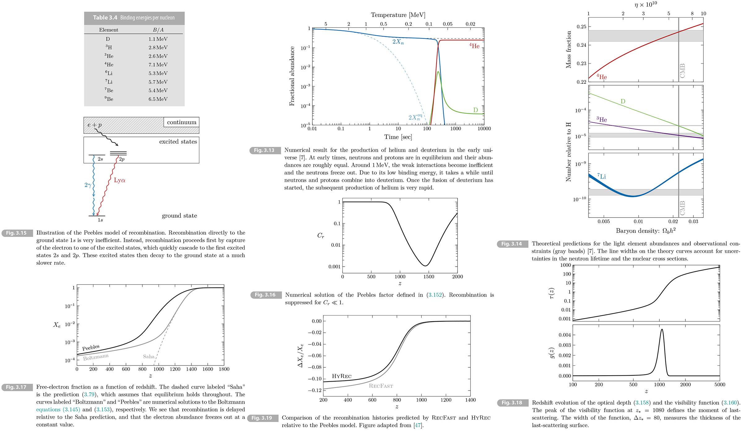
At this point, the universe is mostly protons and neutrons. The first nucleus to form via reaction in (3.117), 𝑛 + 𝑝+ ⟷ 𝐷 + 𝛾, is deuterium.22 Only when deuterium is available can helium be produced. Since deuterium is formed directly from neutrinos and protons it can follow its equilibrium abundance as long as enough free neutrons are available. However, since the deuterium binding energy is rather small (see Table 3.4), it takes a while for the its abundance to become large. Although heavier nuclei have larger binding energies and hence would have larger equilibrium abundance, they cannot be formed until sufficient deuterium has become available. This is the deuterium bottleneck.23 To get a rough estimate for the time of nucleosynthesis, we determine the temperature 𝛵nuc when the deuterium fraction in equilibrium would be of order one, (𝑛𝐷/𝑛𝑝)eq ~ 1.
Deuterium is produced by the reaction in (3.117). Since 𝜇𝛾 = 0, where we have 𝜇𝑛 + 𝜇𝑝 = 𝜇𝐷. To remove the dependence of on the chemical potential, we consider
(3.134) (𝑛𝐷/𝑛𝑛𝑛𝑝)eq = 3/4 (𝑚𝐷/𝑚𝑛𝑚𝑝 2π/𝛵)3/2 𝑒-(𝑚𝐷 - 𝑚𝑛 - 𝑚𝑝)/𝛵, [RE (3.71) 𝑛𝑖eq = 𝑔𝑖 (𝑚𝑖𝛵/2π)3/2 exp[(𝜇𝑖 - 𝑚𝑖)/𝛵.]
where we have used (3.71) with 𝑔𝐷 = 3 and 𝑔𝑝 = 𝑔𝑛 = 2. [𝑔𝐷/𝑔𝑛𝑔𝑝 = 3/4)] In the prefactor 𝑚𝐷 can be set equal to 2𝑚𝑛 ≈ 2𝑚𝑝 ≈ 1.9 GeV, but in the exponential the small deference between 𝑚𝑛 + 𝑚𝑝 and 𝑚𝐷 is crucial: it is the binding energy of deuterium
(3.135) 𝛣𝐷 ≡ 𝑚𝑛 + 𝑚𝑝 - 𝑚𝐷 = 22.2 MeV.
(3.136) (𝑛𝐷/𝑛𝑝)eq = 3/4 𝑛𝑛eq (4π/𝑚𝑝𝛵)3/2 𝑒𝛣𝐷/𝛵.
To get an order-of-magnitude estimate, we approximate the neutron density by the baryon density and write this in terms of the photon temperature and the baryon-to-photon ratio, [RE (3.76) 𝑛𝑏 = 𝜂 𝑛𝛾 = 𝜂 × 2𝜁(3)/π2 𝛵3,]
(3.137) 𝑛𝑛 ~ 𝑛𝑏 = 𝜂 𝑛𝛾 = 𝜂 × 2𝜁(3)/π2 𝛵3.
(3.138) (𝑛𝐷/𝑛𝑝)eq ≈ 𝜂 (𝛵/𝑚𝑝)3/2 𝑒𝛣𝐷/𝛵. [RE 3/4 2𝜁(3)/π2 𝛵3 (4π/𝑚𝑝𝛵)3/2 ≈ 8.14 (𝛵/𝑚𝑝)3/2]
As in the case of recombination, the smallness of baryon-to-photon ratio 𝜂 inhibits the production of deuterium until the 𝛵 drops well below binding energy 𝛣𝐷. The 𝛵 has to drop enough so that 𝑒𝛣𝐷/𝛵 can compete with 𝜂 ≈ 6 × 10⁻¹⁰. We find (𝑛𝐷/𝑛𝑝)eq ~ 1 at 𝛵nuc ~ 0.06 MeV, which via (3.56), [When 𝑎 ∝ 𝑡-1/2, we have 𝐻 = 1/(2𝑡) and the Friedmann equation leads to 𝛵/1MeV ≃ 1.5 𝑔*-1/4(1sec/𝑡)-1/2], with 𝑔* = 3.38 [Dodelson p.67 neutron day (𝑛 → 𝑝 + 𝑒 + 𝜈) and deuterium production (𝑛 + 𝑝 → 𝐷 + 𝛾). When neutrons decay electrons and positrons have annihilated, so 𝑔* = (𝑔result/𝑔𝑛) = [2(𝛾) + 7/8 {3(𝐷) + 𝑓d × 2(𝜈)}]/ [7/8 2(𝑛)] = 2.64 + 𝑓d ≈ 3.38, with decay factor 𝑓d = 0.74.], translates into
(3.139) 𝑡nuc = 120 s (0.1 MeV/𝛵nuc)2 ~ 330 s.
We see from Fig. 3.13 that a better estimate would be 𝑛𝐷eq(𝛵nuc) ≈ 10-3𝑛𝑝eq(𝛵nuc), which gives 𝛵nuc ≈ 0.07 MeV and 𝑡nuc ≈ 250 s. Notice that 𝑡nuc ≪ 𝜏𝑛, so the result for 𝑋𝑛(𝑡nuc) from (3.133) won't be very sensitive to the estimate for 𝑡nuc. Once the fusion of deuterium has started, the subsequent production of helium is very rapid.
Helium
Since the binding energy is larger than that of deuterium, the Boltzmann factor 𝑒𝛣/𝛵 favors helium over deuterium. Fog. 3.13 shows that helium is produced almost immediately after deuterium. The reaction proceeds in two steps: First, helium-3, 3𝐻𝑒, are formed via
𝐷 + 𝑝+ ⟷ 3𝐻𝑒 + 𝛾, 𝐷 + 𝐷 ⟷ 3𝐻 + 𝑝+, 𝐷 + 𝐷 ⟷ 3𝐻𝑒 + 𝑛.
The rate of 𝐷-𝐷 fusion is much faster, but there are more protons than deuterium. Next, helium-4, 4𝐻𝑒, is produced through the following chain of reactions
3𝐻 + 𝑝+ ⟷ 3𝐻 + 𝑛, 3𝐻 + 𝐷 ⟷ 4𝐻𝑒 + 𝑛, 3𝐻 + 𝐷 ⟷ 4𝐻𝑒 + 𝑝+.
Virtually, all the neutrons at 𝑡 ~ 𝑡nuc are processed into 4𝐻𝑒 by these reactions. Substituting 𝑡nuc ≈ 250 s into (3.133), [𝑋𝑛(𝑡) = 𝑋𝑛∞ 𝑒-𝑡/𝜏𝑛 ≈ 0.15 𝑒-𝑡/887 s], we get
(3.140) 𝑋𝑛(𝑡nuc) ≈ 0.11. [RE Dodelson p.67]
Since two neutrons go into one nucleus of 4𝐻𝑒, the final helium abundance is equal to half of the neutron abundance at 𝑡nuc, so that 𝑛𝐻𝑒 = 1/2 𝑛𝑛(𝑡nuc. Hence, the mass fraction of helium is
(3.141) 𝑌𝑃 = 𝑛4𝐻𝑒/𝑛𝐻 = 𝑌𝑃 = 𝑛4𝐻𝑒/𝑛𝑝 = 2𝑋𝑛(𝑡nuc/(1 - 𝑋𝑛(𝑡nuc) ~ 0.25, [= 1/4]
as we wish to show. A more accurate calculation gives [Ref.3-31]
(3.142) 𝑌𝑃 = = 0.2262 + 0.0135 ln(𝜂/10-10,
where the logarithmic dependence on 𝜂 can be trace back to the effect of baryon-to-photon ratio on the time of nucleosynthesis in (1.139). Fig. 3.14 shows the predicted helium mass fraction as a function of 𝜂. The abundance of 4𝐻𝑒 increases with increasing 𝜂 because nucleosynthesis starts earlier for larger baryon density.
In making the prediction (3.141), we have taken the effective number of relativistic species, 𝑔*, to be fixed at the value by the Standard Model. It is also interesting to let the value of 𝑔* float and use measurement to put constraints on any new physics contributing to 𝑔* at BBN. The dependence on 𝑔* is through 𝐻 ∝ √𝑔* 𝛵2, so that increasing the value of 𝑔* leads to a larger expansion rate (at the same 𝛵) which implies an earlier neutron freeze-out, 𝛵𝑓 ∝ 𝑔*1/6.[verification. needed]4𝐻𝑒.
Other light elements
To determine the abundances of other light elements, the coupled Boltzmann equations have to be solved numerically. A qualitative discussion of the most important reactions will just be provided. Wee see in Fig. 3.13 that most of deuterium is processed into 3𝐻𝑒 and 4𝐻𝑒. (Tritium is unstable and decay into 3𝐻𝑒.) The final abundance of 𝐷 and 3𝐻𝑒, as a function of 𝜂, are shown in Fig. 3.14. Since both of them are burnt by fusion, their abundance decrease as 𝜂 increases.
Nucleosynthesis is a very inefficient process, so very few nuclei beyond helium are formed. Small amount of beryllium and lithium are created by the reactions
3𝐻𝑒 + 4𝐻𝑒 ⟷ 7𝛣𝑒 + 𝛾, 3𝐻𝑒 + 4𝐻𝑒 ⟷ 7𝐿𝑖 + 𝛾,
and can be converted via 7𝛣𝑒 + 𝑛 ⟷ 7𝐿𝑖 + 𝑝+.
Lithium can be destroyed by capturing a proton
7𝐿𝑖 + 𝑝+ ⟷ 4𝐻𝑒 + 4𝐻𝑒.
This last reaction reduces the amount of lithium relative to beryllium. However, once the temperature gets low enough, beryllium can decay into lithium by capturing an electron
7𝛣𝑒 + 𝑒- ⟷ 7𝐿𝑖 + 𝜈𝑒,
The predicted amount of lithium is shown in Fig. 3.14. At low 𝜂, 7𝐿𝑖 is destroyed by protons with an efficiency. On the other hand, its precursor 7𝛣𝑒 is produced more efficiently as 𝜂 increases. This explains the valley in the curve for 7𝐿𝑖.
Almost no nuclei with mass number 𝛢 > 7 are produced in the Big Bang. The basic reason is that there are no stable nuclei with 𝛢 = 8 that can be formed fast enough to sustain the chain reaction. The half-life of 8𝛣𝑒 is 10-12 s.The merger of three helium-4 nuclei into carbon-12 is too slow. Similarly the capture of neutrons and protons into 8𝐿𝑖 and 9𝛣𝑒 is very inefficient.
Observations
To test the predictions of Big Bang nucleosynthesis, the element abundances must be measured in the region where very little post-processing of the primordial gas has taken to place. In particular, nuclear fusion inside of stars changes the abundances. The measurements cited below are those suggested by the Particle Data Group [Ref. 3-33]. The fact that we find good quantitative agreement with observations remains one of the great triumphs of the Big Bang model.
• Hellium-4 can be measured from the light of ionized gas clouds, because the strength of some emission lines depends on the amount of helium. We have to correct for the fact that 4𝐻𝑒 is also produced in stars. One way to do this is to correlate the measured helium abundance with the abundances of heavier elements, such as nitrogen and oxygen. The larger the amount of oxygen, the more helium has been created. Extrapolating the measurements to zero oxygen gives an improved estimate of the primordial helium abundance. Using this approach, the measured abundance of primordial helium-4 is found to be [34-36].
(3.143) 𝑌𝑃 = 0.245 ± 0.003.
We see from Fig. 3,14 that this is consistent with the prediction from BBN, given the CMB measurement of the baryon density.
• Deuterium is weakly bound and therefore easily destroyed in the late universe. BBN is the only source of significant deuterium in the universe. The best way to determine the primordial (unprocessed) value of the deuterium abundance is to measure the spectra of high-redshift quasars. These spectra contain absorption lines due to gas clouds along the line-of-sight, and in particular, the Lyman-𝛼 line is a sensitive probe of the amount of deuterium (see e.g. [37]). A weighted mean of several such measurements is 𝐷/𝐻 = (25.47±0.25) × 10-6 [33]. In Fig. 3.14 this agrees precisely with the prediction from BBN.
• Helium-3 can be created and destroyed in stars.In abundance is therefore hard to measure and interpret. Given these uncertainties, helium-3 is usually not used as a cosmological probe,
• Lithium is mostly destroyed by stellar nucleosynthesis. The best estimate of its primordial abundance follows from the measurement of metal-poor stars in the Galactic halo. Averageing the measurements of [38-41] gives 𝐿𝑖/𝐻 = (1.6±0.3) × 10-10. As we see from Fig. 3.14, the measured lithium abundance is significantly smaller than all the predicted value. It is unclear whether this lithium problem is due to systematic errors in the interpretation\n of the measurements or signals the need for new physics during BBN.
3.2.5 Recombination Revisited*
Finally, we will use the Boltzmann equation to provide a more accurate treatment of recombination. It's important to determine the evolution of free-ectron density accurately because it affects the prediction for the CMB anisotropy (see Chapter 7). We assumed previously that thermal equilibrium holds throughout the process. In reality, this assumption breaks down rather quickly and non-equilibrium effects become important. As we will see, recombination directly to the ground state of the hydrogen atom is very inefficient and a more complicated path needs to be considered for the era of precision cosmology.
Non-equilibrium recombination
As thr free-electron fraction drops during recombination, the interaction rate also decreases and can fall below the expansion rate of the universe. When this happens, we must use Boltzmann equation to follow the evolution. Applying (3.96(), 1/𝑎3 𝑑(𝑛1𝑎3)/𝑑𝑡 = -⟨𝜎𝑣⟩ [𝑛1𝑛2 - (𝑛1𝑛2/𝑛3𝑛4)eq 𝑛3𝑛4], to the reaction 𝑒- + 𝑝+ ⟷ 𝐻 + 𝛾, we get
(3.144) 1/𝑎3 𝑑(𝑛𝑒𝑎3)/𝑑𝑡 = -⟨𝜎𝑣⟩ [𝑛𝑒2 - (𝑛𝑒2/𝑛𝐻)eq𝑛𝐻],
where we have used that 𝑛𝑒 = 𝑛𝑝 and 𝑛𝛾 = 𝑛𝛾eq. For the factor of (𝑛𝑒2/𝑛𝐻)eq we can use (3.74), (𝑛𝐻/𝑛𝑒2)eq = (2π/𝑚𝑒𝛵)3/2 𝑒𝐸𝐼/𝛵. Moreover, the electron and hydrogen densities can be written as, 𝑛𝑒 = 𝑋𝑒𝑛𝑏 and 𝑛𝐻 = (1 - 𝑋𝑒) 𝑛𝑏.
Using that 𝑛𝑏𝑎3 = const, we then get
(3.145) 𝑑𝑋𝑒/𝑑𝑡 = [𝛽(𝛵) (1 - 𝑋𝑒) - 𝛼(𝛵)𝑛𝑏𝑋𝑒2],
where we have introduced
(3.146-7) 𝛼(𝛵) ≡ ⟨𝜎𝑣⟩, 𝛽(𝛵) ≡ ⟨𝜎𝑣⟩ (𝑚𝑏𝛵/2π)3/2 𝑒-𝐸𝐼/𝛵.
The parameter 𝛼 characterizes the recombination rate, while 𝛽 is associated with the ionization rate. When 𝛼 is large, right-hand side of (3.145) must vanish and the evolution of 𝑋𝑒 is given by Saha equilibrium. The function 𝛼(𝛵) depends on the precise way that the electrons get captured into the ground state, it releases photons with energy larger than 13.6 eV. These photons will then quickly ionized other atoms, leading to no net recombination.
The effective three-level atom
To avoid the instantaneous reionization of the hydrogen atoms, recombination must first to an excited state, which then decays to the ground state. The photon created during this multi-step recombination have lower energy and are therefore less likely to ionize the hydrogen atoms. The details were worked out by Peebles in 1968 [43] (see also Zel'dovich, Kurt and Sunyaev [43]).
Peebles first argued That the hydrogen atom can be treated as an effective three-level atom. The three relevant states are the ground state (1𝑠), the excited states (mostly 2𝑠 and 2𝑝), and the continuum states of ionized hydrogen (see Fig. 3.15). The excited states are in thermal equilibrium with each other since radiative excitations and decays are very fast. Peebles therefore considered all excited states as a single entity.Since the direct recombination to the ground state is very inefficient, the rate of recombination will be determined by the rate of decayof the first excited state. A standard computation in quantum field theory gives [Dodelson p.71]
(3.148) 𝛼(𝛵) ≈ 9.8 𝛼2/𝑚𝑒2 (𝐸𝐼/𝛵)1/2 ln (𝐸𝐼/𝛵),
where 𝛼 ≈ 1/137 is the fine-structure constant.
But, this is still bot the answer. When an atom in the first excited state decays to the ground state, it produces a Lyman-𝛼 photon. This photon has a large probability to be absorbed by a near by atom. which can then be ionized.To achieve a significant level of recombination we must avoid these resonant excitation. There are two way out:
• First, there is a small probability that the 2𝑠 state will decay to the 1𝑠 state through the emission of two photons. These photons then don't have enough energy to excite the atoms in the ground state back to the first excited state. The rate for this two-photon decay is
(3.149) 𝛬2𝜆 = 8.227 s-1.
About 57% of all natural hydrogen is formed via this route.
• Second, as the universe expands, the energy of the Lyman-𝛼 photons that are created by the 2𝑝 → 1𝑠 transition is redshifted. This moves these photons off resonance. If a photon avoids being reabsorbed for a sufficiently long time, then this effect allows them to escape. There is a small probability that this will happen. The rate of recombination via this resonance escape is [44].24
(3.150) 𝛬𝛼 = 8π/𝜆𝑎3𝑛1𝑠 𝐻,
where 𝜆𝑎 ≡ 2π𝐸𝛼-1 = 8π/(3𝐸𝐼) is the wavelength of a Lyman--𝛼 photon and 𝑛1𝑠 ≈ (1 - 𝑋𝑒)𝑛𝑏 is the abundance of hydrogen atoms in the 1𝑠 state. Substituting 𝑛𝑏 = 𝜂 𝑛𝛾, the recombination rate becomes
(3.151) 𝛬𝛼 = 27/[128𝜁(3)] 𝐻(𝛵)/[(1 - 𝑋𝑒) 𝜂 (𝛵/𝐸𝐼)3].
About 43% of all hydrogen atoms are formed in this way.
Although the details of the details of the analysis are rather complex, the final answer is easy to state and interpret.The main new parameter is the effective branching ratio
(3.152) 𝐶𝑟(𝛵) ≡ (𝛬2𝜆 + 𝛬𝛼)/(𝛬2𝜆 + 𝛬𝛼 + 𝛽𝛼),
where 𝛽𝛼 ≡ 𝛽𝑒3𝐸𝐼/4𝛵 is the ionization rate of the 𝑛 = 2 state. 𝐶𝑟 will be called Peebles factor. It describe the probability that an atom in the first excited state reaches the ground state through either of the two ways described above before being ionized. When 𝐶𝑟 is much smaller than unity, recombination is suppressed. The evolution of 𝐶𝑟(𝑧) is shown in Fig. 3.16. We see that 𝐶𝑟 ≪ 1 for 𝑧 > 900, which implies that recombination will be delayed.
The branching ratio 𝐶𝑟 appears as a multiplicative factor in the evolution equation (3.145), leading to the so-called Peebles equation
(3.153) 𝑑𝑋𝑒/𝑑𝑡 = 𝐶𝑟 [𝛽(𝛵) (1 - 𝑋𝑒) - 𝛼(𝛵)𝑛𝑏𝑋𝑒2].
This equation can be integrated numerically to obtain the evolution of free-electron fraction.
Electron freeze-out
It will be convenient to use redshift instead of timeas the indipendent variable during the evolution. Using [(2.63) 𝑎 = (1 + 𝑧)-1, 𝐻 = 1/𝑎 𝑑𝑎/𝑑𝑡 = (1 + 𝑧) 𝑑 (1 + 𝑧)-1/𝑑𝑡 = (1 + 𝑧) × -(1 + 𝑧)-2 𝑑𝑧/𝑑𝑡 = -(1 + 𝑧)-1 𝑑𝑧/𝑑𝑡. ⇒ 𝑑𝑧/𝑑𝑡 = -(1 + 𝑧) 𝐻. ▮)
(3.154) 𝑑𝑋𝑒/𝑑𝑡 = 𝑑𝑋𝑒/𝑑𝑧 𝑑𝑧/𝑑𝑡 = -𝑑𝑋𝑒/𝑑𝑧 𝐻(1 + 𝑧),
the Peebles equation (3.153) can then be written as
(3.155) 𝑑𝑋𝑒/𝑑𝑧 = -𝐶𝑟(𝑧)/𝐻(𝑧) 𝛼(𝑧)/(1 + 𝑧) [(1 - 𝑋𝑒) (𝑚𝑏𝛵/2π)3/2 𝑒-𝐸𝐼/𝛵 - 𝑋𝑒2 𝜂 2𝜁(3)/π2 𝛵3],
where 𝛵 = 0.235 meV (1 + 𝑧). The evolution of the Hubble parameter is
(3.156) 𝐻(𝑧) = √𝛺𝑚 𝐻0 (1 + 𝑧)3/2 [1 + (1 + 𝑧)/(1 + 𝑧eq)]1/2,
with 𝐻0 ≈ 1.5 × 10⁻³³ eV. Fig. 3.17 shows the evolution of the free-electron fraction as a function of redshift. We see that recombination is indeed delayed relative to the Saha expectation. In particular, 𝑋𝑒 = 0.5 at 𝑧 = 1270 (compared to 𝑧 = 1380 for Saha.) Unlike the Saha prediction the electron density freeze out at a non-zero value about 2 × 10⁻⁴.
Decoupling and last-scattering
In Section 3.1.5, we defined last-scattering as the moment when the optical depth, (𝑡* ≡ 1. The probability that a photon did not scatter off an electron in the redshift interval [𝑧0, 𝑧1] is,
(3.157) 𝑃(𝑧0, 𝑧1) = 𝑒-𝜏(𝑧0,𝑧1))
where 𝜏 is the optical depth
(3.158) 𝜏(𝑧0, 𝑧1) ≡ ∫𝑡1𝑡0 𝑑𝑡 𝜎𝛵 𝑛𝑒(𝑡) = ∫𝑧0𝑧1 𝑑𝑧 𝜎𝛵 𝑛𝑏𝑋𝑒(𝑧)/[𝐻(1 + 𝑧)].
The probability that a photon scattered for the last time in the interval [𝑧1, 𝑧1 + 𝑑𝑧1] then is
(3.159) 𝑃(𝑧0, 𝑧1) - 𝑃(𝑧0, 𝑧1 + 𝑑𝑧1) ≡ 𝑔(𝑧0, 𝑧1) 𝑑𝑧1, where 𝑔(𝑧0, 𝑧1) is the visibility function. We will be interested in 𝑔(𝑧) ≡ (0, 𝑧), which which is the probability that a photon observed today scattered last at redshift 𝑧. Using (3.157) and (3.159), we have25
(3.160) 𝑔(𝑧) = -𝑑/𝑑𝑧 𝑒-𝜏(0,𝑧) = 𝑑𝜏/𝑑𝑧 𝑒-𝜏
Note that 𝜏(0, 0) = 0 and 𝜏(0, ∞) = ∞, so that the visibility function satisfies
(3.161) ∫0∞ 𝑑𝑧 𝑔(𝑧) = -𝑒-𝜏∣0∞ = 1.
as required for a probability density. At early times, 𝜏 is large and the visibility function is exponentially suppressed. After combination, 𝑑𝜏/𝑑𝑧 is small because the density of free electrons small. This means that 𝑔(𝑧) will be pealed at the moment of decoupling. Indeed, this is what find in Fig. 3.18. The maximum of the visibility function is at 𝑧* = 1080, which we take as our definition of the moment of last-scattering. The function has a width of 𝛥𝑧* = 80, which characterizes the finite width of the last-scattering surface.
Precision cosmology
It is remarkable how much of the comp;ex physics of recombination was understood by Peebles and others in the 1960s. For the analysis of modern CMB experiments, however, the above analysis is still not enough.The most imortant
development of refined analysis of recombination will be sketched, since they made the modern era of precision cosmology possible.
The three-level atom assumes that all excited staes are equilibrium with the 𝑛 = 2 staes. This assumption breaks down during the later stages of precise multi-level atom was first studied by Seager, Sasselov and Scott in 1999 [46].
It was found that accounting for the additional excited states leads to an increase in the rate of recombination in the late times (see Fig. 3.19). To follow the evolution of each state, a large number of coupled Boltzmann equation has to be solved. Fortunately, the dynamics can be mimicked by solving it with an an enhanced recombination coefficient 𝛼 → 1.14 𝛼. This approach became the basis of the recombination code RECFAST.
While RECFAST was precise unbiased analysis of the enough for the analysis of the WMAP data, an unbiased analysis of the Planck data required konwing the recombination history to better than 0.1%. many new effects were identified that change the predictions at the 1% level and therefore needed to to be included in the analysis:
• Seager et al. [46] assumed that states with same energy, but different angular momentum quantum number 𝓁, were in equilibrium. This assumption breaks down at the percent level [48]. As in the original analysis of Seager et al., solving for the abundances of all the excited states at every time-step is numerically very expensive. An elegant solution to this problem was found by Ali-Haimoud and Hirata [49]. They realized only the populations of a few excited states had to be tracked, provided one uses precomputed effective states of hydrogen. This effective multi-level atom is the basis of the recombination codes HYREC [47] and COSMOREC [50].
• At the precision of the Planck experiment, the rates for these processes have to be modeled more accurately than we have done. For example, stimulated two-photon emission cannot be ignored and changes the effective two-photon decay rate 𝛬2𝛾 at the percent level [51]. Similarly, the absorption of non-thermal photons (produced in previous transitions) must be accounted for [52]. More generally, the time dependent radiative transfer problem must be solved to high accuracy; see [53-57] for further relevant corrections. Finally, it was realized that two-photon decay from higher excited states, 𝑛𝑠 and 𝑛𝑑, become relevant at this level of accuracy [58-60].
3.3 Summary
In this chapter, we have studied the thermal history of the universe. At early times, the rates of particle interactions, 𝛤, were much larger than the expansion rate, 𝐻, so that all particles were in equilibrium at a common temperature, 𝛵. The energy density was dominated by relativistic species
(3.162) 𝜌 = π 2/30 𝑔*𝛵4,
where 𝑔* is the effective number of relativistic degrees of freedom (which is the sum of the internal degrees of freedom for each particle weighted by a factor of 7/8 for fermions). The pressure of the primordial plasma was 𝑃 = 𝜌/3, so that it behaved like radiation.
An important quantity is the entropy density
(3.163) 𝑠 = (𝜌 + 𝑃)/𝛵 = 2π2/45 𝑔*𝑆𝛵3
where 𝑔*𝑆 is the effective number of relativistic degrees of freedom in entropy which for most of the universe's history was equal to 𝑔*. The conversation of entropy then implies 𝑔*𝑆𝛵3 ∝ 𝑎3 . We used this to relate the temperature of the cosmic neutrino background to that of the cosmic microwave background 𝛵𝑣 = (4/11)1/3𝛵𝛾.
To study non-equilibrium effects, we introduced the Boltzmann equation. For processes of the form 1 + 2 ⟷ 3 + 4, the Boltzmann equation for the species 1 can be written as
(3.164) 𝑑 ln 𝑁1/𝑑 ln 𝑎 = -𝛤1/𝐻 [1 - (𝑁1𝑁2/𝑁3𝑁4)eq 𝑁3𝑁4/𝑁1𝑁2],
where 𝑁𝑖 = 𝑛𝑖/𝑠 is proportional to the number of particles in comoving volume. As long as the interaction rate is larger than the expansion rate, 𝛤1 ≫ 𝐻, the particle abundance tracks its equilibrium value. Once the interaction rate drops below the expansion rate, however, the particles drop out of thermal equilibrium and decouple from the thermal bath. by integrating the Boltzmann equation, we can follow the non-equilibrium evolution of the particle abundances. We presented three examples: (i) dark matter freeze-out (ii) Big Bang nucleosynthesis; and (iii) recombination.
As a simple example of dark matter production, we considered the reaction 𝑋 + 𝑋̄ ⟷ 𝓁 + 𝓁̄, We used the Boltzmann equation to follow the evolution of the density of dark matter particles 𝑋. The resulting dark matter density today depends inversely on the annihilation cross section.
We then studied nucleosynthesis. Initially, the most abundant nuclei were neutrinos and protons, kept in equilibrium through reactions of the form
𝑛 + 𝜈𝑒 ⟷ 𝑝+ + 𝑒-.
Around 1 MeV, these reactions become inefficient and the neutrons decoupled. We derived the freeze-out abundance by solving the Boltzmann equation. At 0.1 MeV, neutrinos and protons fused into deuterium, which then combined with protns into helium-3 and helium-4:
𝑛 + 𝑝+ → 𝐷 + 𝛾, 𝐷 + 𝑝+ → 3𝐻𝑒 + 𝛾, 𝐷 + 3𝐻𝑒 → 4𝐻𝑒 + 𝑝+.
The resulting mass fraction of helium-4 is 𝑌𝑃 ≡ 𝑛4𝐻𝑒/𝑛𝐻 ≈ 0.25, with a weak dependence on the baryon density of the universe.
Finally, we investigate the recombination reaction
𝑒- + 𝑝+ → 𝐻 + 𝛾.
We used the Boltzmann equation to follow the evolution of the free-electron fraction, 𝑋𝑒 ≡ 𝑛𝑒/𝑛𝑏. We took into account that recombination directly to the ground state is very inefficient and instead proceeds via two-photon decay and resonance escape from the first excited state. Defining recombination as the time when 𝑋𝑒 = 0.5, we found
(3.165) 𝑧rec ≈ 1270, 𝑡rec ≈ 290 000 yrs.
As the number of free electron dropped, the reaction 𝑒- + 𝛾 ⟷ 𝑒- + 𝛾 became inefficient and the photons decoupled. This happened at
(3.166) 𝑧dec ≈ 1090, 𝑡dec ≈ 370 000 yrs.
The photons from this era are observed today as the CMB.
22 The fusion of two protons is inefficient because the nuclei have to overcome the Coulomb repulsion before the nuclear force can take over. The fusion of two neutrons produces a very unstable nucleus.
23 Even in equilibrium the production of helium would rather late, at 𝛵 ~ 0.3 MeV. The deuterium bottleneck leads to a further delay of this equilibrium expectation.
24 This rate is a product of rate of the decay 2𝑝 → 1𝑠 + 𝛾 and the probability that the Lyman-𝛼 photon escapes to infinity without exciting another hydrogen atom. We cna find a more detailed discussion on Peebles' orginal paper {42] or in Weinberger's book [45: Weinberger]
25 In Chaper 7, we will define the visibility function in terms of conformal time, 𝑔(𝑧) ≡ (𝑒-𝜏)' = -𝜏' 𝑒-𝜏, where ' ≡ ∂𝜂. In that case, its peak is at 𝑧* = 1090. |
|
|