|
김관석
|
2024-12-18 11:51:05, 조회수 : 62 |
- Download #1 : BC_8a.jpg (117.1 KB), Download : 0

8 Quantum Initial Conditions
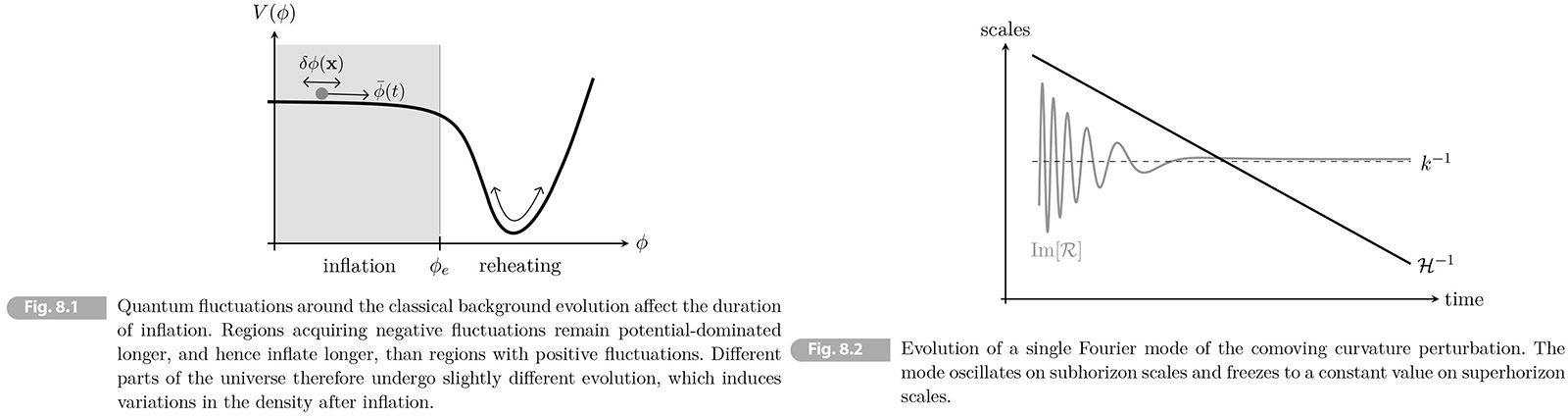
One of the most remarkable features of inflation is that it provides a natural mechanism for creating the primordial density fluctuations that seeded the structure in the universe. Recall that the evolution of the inflaton field 𝜙(𝑡) governs the energy density of the early universe 𝜌(𝑡) and hence, controls the end of inflation (see Fig. 8.1). Essentially, the field 𝜙 plays the role of a "clock" telling us the amount of inflationary expansion still remaining. However, by the uncertainty principle, arbitrary precise timing is impossible in quantum mechanics. Instead, quantum mechanical clocks necessarily have some variance, so the inflaton will therefore varaying fluctuations 𝛿𝜙(𝑡, 𝐱). The time at which inflation ends will therefore vary across space. Although these fluctuations are a small quantum effect, they trigger large differences in the local expansion histories, which lead to significant differences in the local densities after inflation, 𝛿𝜌(𝑡, 𝐱). Regions of space that end inflation first will start diluting and therefor end up having smaller densities, while regions that inflate for a longer time will have higher densities. It is worth emphasizing that the theory was not engineered to produce these fluctuations, but that their origin is instead a natural consequence of treating inflation quantum mechanically.
In this chapter we will derive the spectrum of quantum fluctuations produced during inflation. We will begins, in Section 8.1 by deriving the classical equations of motion of the inflation fluctuations in spatially flat gauge. We will find that each Fourier mode satisfies the equation of a harmonic oscillator with a time-dependent frequency. In Section 8.2 we will show how quantum zero-point fluctuations after inflation, becoming the seeds for all structure in the universe. We will derive the forms of the primordial scalar and tensor power spectra, and relate these predictions to the shape of the inflation potential in slow-roll models. In section 8.4 we will present current observational constraints on inflationary models and comment on the prospects for future tests.
For pedagogical reasons the presentation will focus on single-field slow-roll models of inflation. It is important to appreciate that the landscape of inflationary models is much larger and there are many different mechanisms that can produce the inflationary expansion of the spacetime (see e.g. [1] for a review). An interesting way of describing a large class of models is in terms of an effective theory of the inflationary fluctuations. Given a suitable Hubble parameter 𝐻(𝑡) (whose origin doesn't have to be specified), we can construct an effective theory for the associated Goldston boson of spontaneously broken time translations. On superhorizon scales, this Goldstone boson is closely related to the primordial curvature perturbations and adiabatic density fluctuations.[verification needed] By focusing directly on the inflationary fluctuations, this EFT of inflation provides an effective way of describing the prediction of inflation [2]. The quantization procesure described inthis chapter for slow-roll inflation applies straightfowardly in broader context.
8.1 Inflationary Perturbations
The dynamics of the inflaton field is determined by the following action
(8.1) 𝑆 = ∫ d4𝑥√-𝑔 [-1/2 𝑔𝜇𝜈∂𝜇𝜙∂𝜈𝜙 - 𝑉(𝜙)].
where 𝑔 ≡ det(𝑔𝜇𝜈) (see Appendix A). The coupling to the metric will lead to a nontrivial mixing between the inflaton fluctuations 𝛿𝜙 and the metric fluctuations 𝛿𝑔𝜇𝜈. The form of this mixing is gauge dependent. Foe example in comoving gauge the inflaton fluctuation vanish, 𝛿𝜙 ≡ 0. and all fluctuations arein metric. To make contact with the intuitive picture of inflaton fluctuation shown in Fig. 8.1, however, it will instead be convenient to work in the spatially flat gauge, where the line element (with scalar fluctuations) takes form
(8.2) d𝑠2 = 𝑎(𝜂) [-(1 + 2𝛢)d𝜂2 + 2∂𝑖𝛣d𝑥𝑖d𝜂 + 𝛿𝑖𝑗d𝑥𝑖d𝑥𝑗].
The metric fluctuation 𝛢 and 𝛣 are related to the inflaton fluctuations 𝛿𝜙 through the Einstein equations, leaving a single degree of freedom to describe the inflationary fluctuations. We will begin by deriving the classical equation of motion for 𝛿𝜙 and then discuss its quantization.
8.1.1 Equation of Motion
Varying of the action (8.1) leads to Klein-Gordon equation for the inflation field.
(8.3) 1/√-𝑔 ∂𝜇(√-𝑔 𝑔𝜇𝜈∂𝜈𝜙) = 𝑉,𝜙,
where 𝑉,𝜙 ≡ d𝑉/d𝜙.
Exercise 8.1 Show that (8.3) follows from (8.1).
[Solution] Varying the action with respect to 𝜙, we get
(a) 𝛿𝑆 = ∫ d4𝑥√-𝑔 (-𝑔𝜇𝜈∂𝜇𝛿𝜙∂𝜈𝜙 - 𝑉,𝜙𝛿𝜙) = ∫ d4𝑥√-𝑔 [1/√-𝑔 ∂𝜈(√-𝑔 𝑔𝜇𝜈 ∂𝜇𝜙) - 𝑉,𝜙]𝛿𝜙.
Since the principle of least action states 𝛿𝑆 = 0, for arbitrary 𝛿𝜙 the expression in the square brackets must vanish. So we find
(b) 1/√-𝑔 ∂𝜈(√-𝑔 𝑔𝜇𝜈 ∂𝜇𝜙) - 𝑉,𝜙 = 0. ⇒ 1/√-𝑔 ∂𝜈(√-𝑔 𝑔𝜇𝜈 ∂𝜇𝜙) = 𝑉,𝜙. ▮
At first order in the fluctuations, the components of the inverse metric are
(8.4) 𝑔00 = -𝑎-2(1 - 2𝛢), 𝑔0𝑖 = 𝑎-2∂𝑖𝛣, 𝑔𝑖𝑗 = 𝑎-2𝛿𝑖𝑗,
and √-𝑔 = 𝑎4(1 + 𝛢). Substituting the perturbed field 𝜙 = 𝜙̄ + 𝛿𝜙 and the perturbed metric (8.2) into the equation of motion (8.3), we get
(8.5) 𝛿𝜙ʺ + 2𝓗𝛿𝜙ʹ - ∇2𝛿𝜙 = (𝛢ʹ + ∇2𝛣)𝜙̇ʹ - 2𝑎2𝑉,𝜙𝛢 - 𝑎2𝑉,𝜙𝜙𝛿𝜙,
where 𝑉,𝜙𝜙 ≡ d2𝑉/d𝜙2.
Exercise 8.2 Show that (8.5) follows from (8.3).
[Solution] The Klein-Gordon equation (8.3) can be written as
(a) ∂𝜇(√-𝑔 𝑔𝜇𝜈∂𝜈𝜙) - 1/√-𝑔 𝑉,𝜙 = 0
The first term can be written as
(b) ∂𝜇(√-𝑔 𝑔𝜇𝜈∂𝜈𝜙) = ∂0(√-𝑔 𝑔00∂0𝜙) + ∂𝑖(√-𝑔 𝑔0𝑖∂0𝜙) + ∂0(√-𝑔 𝑔𝑖0∂𝑖𝜙) + ∂𝑗(√-𝑔 𝑔𝑖𝑗∂𝑖𝜙)
Since ∂𝑖𝜙 = ∂𝑖𝜙𝛿𝜙 can be evaluated using 𝜙 = 𝜙̄ + 𝛿𝜙. Then 𝑔̄𝑖0 = 0, 𝑔̄𝑖𝑗 = 𝑎-2 and √-𝑔̄ = 𝑎4. So we find
(b) ∂𝜇(√-𝑔 𝑔𝜇𝜈∂𝜈𝜙) = ∂0(√-𝑔 𝑔00∂0𝜙) + ∂𝑖(√-𝑔 𝑔0𝑖∂0𝜙) + 𝑎2∇2𝛿𝜙
Since 𝑔0𝑖 = 𝑎-2∂𝑖𝛣, ∂0𝜙 = 𝜙̄ʹ + 𝛿𝜙ʹ and if we neglect 𝑔0𝑖𝛿𝜙ʹ term which is so small, we then have
(c) ∂𝜇(√-𝑔 𝑔𝜇𝜈∂𝜈𝜙) = ∂0(√-𝑔 𝑔00∂0𝜙) + 𝑎2∇2𝛣𝜙̄ʹ + 𝑎2∇2𝛿𝜙.
Substituting (8.4) into the first term in the right-hand side if we also neglect -2𝛢2 term here, we then get
(d) ∂0(√-𝑔 𝑔00∂0𝜙) = ∂0[𝑎4)(1 + 𝛢)(-𝑎-2(1 - 2𝛢)∂0𝜙] = - ∂0[𝑎2(1 - 𝛢)(𝜙̄ʹ + 𝛿𝜙ʹ)] = -∂0(𝑎2𝜙̄ʹ) - ∂0(𝑎2𝛿𝜙ʹ) + ∂0(𝑎2𝜙̄ʹ)𝛢 + 𝑎2𝜙̄ʹ𝛢ʹ,
(e) ∂𝜇(√-𝑔 𝑔𝜇𝜈∂𝜈𝜙) = -∂0(𝑎2𝜙̄ʹ) - ∂0(𝑎2𝛿𝜙ʹ) + 𝑎2∇2𝛿𝜙 + ∂0(𝑎2𝜙̄ʹ)𝛢 + 𝑎2(𝛢ʹ + ∇2𝛣)𝜙̄ʹ.
The second term of (a) with its variation, if we neglect 𝛢𝑉,𝜙𝜙𝛿𝜙 term, can be written
(f) √-𝑔 𝑉,𝜙 = 𝑎4(1 + 𝛢)(𝑉,𝜙 + 𝑉,𝜙𝜙𝛿𝜙) = 𝑎4𝑉,𝜙 + 𝑎4𝑉,𝜙𝛢 + 𝑎4𝑉,𝜙𝜙𝛿𝜙.
Now (a) becomes
(g) 0 = -∂0(𝑎2𝜙̄ʹ) - ∂0(𝑎2𝛿𝜙ʹ) + 𝑎2∇2𝛿𝜙 + ∂0(𝑎2𝜙̄ʹ)𝛢 + 𝑎2(𝛢ʹ + ∇2𝛣)𝜙̄ʹ -𝑎4𝑉,𝜙 - 𝑎4𝑉,𝜙𝛢 - 𝑎4𝑉,𝜙𝜙𝛿𝜙
= -[∂0(𝑎2𝜙̄ʹ) + 𝑎4𝑉,𝜙]- ∂0(𝑎2𝛿𝜙ʹ) + 𝑎2∇2𝛿𝜙 - 𝑎4𝑉,𝜙𝜙𝛿𝜙 + [∂0(𝑎2𝜙̄ʹ) - 𝑎4𝑉,𝜙]𝛢 + 𝑎2(𝛢ʹ + ∇2𝛣)𝜙̄ʹ.
Since the first line is zeroth order in fluctuations and and implies the background equation of motion, we can find
(h) ∂0(𝑎2𝜙̄ʹ) + 𝑎4𝑉,𝜙 = 0 ⇒ 𝜙̄ʺ + 2𝓗𝜙̄ʹ + 𝑎2𝑉,𝜙 = 0.
Finally to find we get
(i) 𝛿𝜙ʺ + 2𝓗𝛿𝜙ʹ - ∇2𝛿𝜙 = (𝛢ʹ + ∇2𝛣)𝜙̄ʹ - 2𝑎2𝑉,𝜙𝛢 - 𝑎2𝑉,𝜙𝜙𝛿𝜙. ▮
Next, we will use the Einstein equations to eliminate 𝛢 and 𝛣 in favor of 𝛿𝜙. One finds
(8.6-7) 𝛢 = 𝜀 𝓗/𝜙̄ʹ 𝛿𝜙, ∇2𝛣 = -𝜀 𝓗/𝜙̄ʹ [𝛿𝜙ʹ + (𝛿 - 𝜀)𝓗𝛿𝜙].
(8.8-9) 𝜀 ≡ - Ḣ/𝐻2 = 1 - 𝓗ʹ/𝓗2 = 4π𝐺 𝜙̄ʹ2/𝓗2, 𝛿 ≡ - (d𝜙̇/d𝑡)/𝐻𝜙̄̇ = 1 - 𝜙̄ʺ/𝓗𝜙̄ʹ.
Despite of the similar appearance we did not make any slow-roll approximation in (8.6-7). Nevertheless it is woth highlighting that the metric perturbations are proportional to the slow-roll parameters, so that the mixing with the inflation fluctuation vanishes at leading order in the slow-roll limit, 𝜀, 𝛿 → 0. This is a special feature of spatially flat gauge. In a general gauge this mixing would be order one in the slow-roll limit. Even in spatially flat gauge, the leading slow-roll correction will play an important role on superhorizon scales.
Derivation Now we will provide some of the intermediate steps of derivation of (8.6-7). First, we consider the 0𝑖 Einstein equation. It takes the form
(8.10) 𝛿𝐺0𝑖 = - 2𝓗/𝑎2 ∂𝑖𝛢 = 8π𝐺 𝛿𝛵0 𝑖 = -8π𝐺 𝜙̄ʹ/𝑎2 ∂𝑖𝛿𝜙,
where the final equality follows from the perturbed energy-momentum tensor of a scalar field (4.53). This implies the result in (8.6):
(8.11) 𝛢 = 4π𝐺 𝜙̄ʹ/𝓗 𝛿𝜙 = 𝜀 𝓗/𝜙̄ʹ 𝛿𝜙.
Next, we look at the 00 Einstein equation,
(8.12) 𝛿𝐺00 = 2𝓗/𝑎2 (3𝓗𝛢 + ∇2𝛣) = 8π𝐺 𝛿𝛵0 0 = -8π𝐺 [𝑎-2(𝜙̄ʹ 𝛿𝜙 - 𝜙̄ʹ2𝛢) + 𝑉,𝜙𝛿𝜙].
Using the background equation of motion
(8.13) 𝜙̄ʺ + 2𝓗𝜙̄ʹ + 𝑎2𝑉,𝜙 = 0,
and the solution (8.11) for 𝛢, we obtain the result (8.7). ▮
Substituting (8.6-7) into (8.5) leads to a closed form equation for the inflation fluctuations:
(8.14) 𝛿𝜙̄ʺ + 2𝓗𝛿𝜙ʹ - ∇2𝛿𝜙 = [2𝜀(3 + 𝜀 - 2𝛿) - 𝑎2𝑉,𝜙𝜙/𝓗2]𝓗2𝛿𝜙.
Note that (𝛢ʹ + ∇2𝛣)𝜙̄ʹ term was canceled so that the mixing with the metric fluctuation only contributes to the effective mass of the inflaton fluctuation. Using the background equation of motion to write 𝑉,𝜙𝜙 in terms of the slow-roll parameters, we find
(8.15) 𝛿𝜙̄ʺ + 2𝓗𝛿𝜙ʹ - ∇2𝛿𝜙 = [(3 + 2𝜀 - 𝛿)(𝜀 - 𝛿) - 𝛿ʹ/𝓗]𝓗2𝛿𝜙.
The friction term 2𝓗𝛿𝜙ʹ can be eliminated by defining the variable
(8.16) 𝑓 ≡ 𝑎𝛿𝜙,
so that
(8.17) 𝛿𝜙̄ʺ + 2𝓗𝛿𝜙ʹ = 1/𝑎 [𝑓ʺ - (2 - 𝜀)𝓗2𝑓].
Collecting all the terms, we find a beautiful equation, the so-called Mukhanov-Sasaki equation:
(8.18) 𝑓ʺ + (𝑘2 - 𝑧ʺ/𝑧)𝑓 = 0, where 𝑧 ≡ 𝑎𝜙̄ʹ/𝓗.
This equation is quite remarkable: it contains the coupling matter and metric fluctuations, does not make any slow-roll approximation, and is valid on all scales. It will be our master equation for the rest of the chaprer.
Exercise 8.4 Fill in the gaps in the derivation of (8.18)
Hints: Show that
(8.19) - 𝑎2𝑉,𝜙𝜙/𝓗2 = (𝛿 - 3)(𝜀 + 𝛿) - 𝛿ʹ/𝓗,
(8.20) 𝑧ʺ/𝑧 = [2 + 2𝜀 - 3𝛿 + (2𝜀 - 𝛿)(𝜀 - 𝛿) - 𝛿ʹ/𝓗]𝓗2.
[Solution] We start from equations (8.5-9), we write again them
(a) 𝛿𝜙ʺ + 2𝓗𝛿𝜙ʹ - ∇2𝛿𝜙 = (𝛢ʹ + ∇2𝛣)𝜙̇ʹ - 2𝑎2𝑉,𝜙𝛢 - 𝑎2𝑉,𝜙𝜙𝛿𝜙, where 𝑉,𝜙𝜙 ≡ d2𝑉/d𝜙2.
(b) 𝛢 = 𝜀 𝓗/𝜙̄ʹ 𝛿𝜙, ∇2𝛣 = -𝜀 𝓗/𝜙̄ʹ [𝛿𝜙ʹ + (𝛿 - 𝜀)𝓗𝛿𝜙].
(c) 𝜀 = 1 - 𝓗ʹ/𝓗2 = 4π𝐺 𝜙̄ʹ2/𝓗2, 𝛿 = 1 - 𝜙̄ʺ/𝓗𝜙̄ʹ.
(d) 𝛢ʹ + ∇2𝛣 = (𝜀 𝓗/𝜙̄ʹ)ʹ𝛿𝜙 - 𝜀 𝓗/𝜙̄ʹ(𝜀 𝓗/𝜙̄ʹ,
(e) (𝜀 𝓗/𝜙̄ʹ)ʹ𝛿𝜙 = (4π𝐺 𝜙̄ʹ2/𝓗2)ʹ 𝛿𝜙 = 4π𝐺 (𝜙̄ʺ/𝓗 - 𝜙̄ʹ𝓗ʹ/𝓗2) 𝛿𝜙 = 4π𝐺 𝜙̄ʹ/𝓗 (𝜙̄ʺ/𝜙̄ʹ𝓗 - 𝓗ʹ/𝓗2) 𝓗𝛿𝜙
= 𝜀 𝓗/𝜙̄ʹ (1 - 𝛿 + 𝜀 - 1) 𝓗𝛿𝜙 = 𝜀 𝓗/𝜙̄ʹ (𝜀 - 𝛿) 𝓗𝛿𝜙.
The first term on the right-hand side of (a) is
(f) (𝛢ʹ + ∇2𝛣)𝜙̄ʹ = 2𝜀(𝜀 - 𝛿) 𝓗2𝛿𝜙.
The second term there is
(g) -2𝑎2𝑉,𝜙𝛢 = 2(𝜙̄ʺ + 2𝓗𝜙̄ʹ) 𝜀 𝓗/𝜙̄ʹ 𝛿𝜙 = 2𝜀 (𝜙̄ʺ/𝓗𝜙̄ʹ + 2) 𝓗2𝛿𝜙 = 2𝜀 (3 - 𝛿) 𝓗2𝛿𝜙.
(h) (𝛢ʹ + ∇2𝛣)𝜙̄ʹ - 2𝑎2𝑉,𝜙𝛢 = 2𝜀 (3 + 𝜀 - 2𝛿) 𝓗2𝛿𝜙.
So equation (a) can be written as
(i) 𝛿𝜙ʺ + 2𝓗𝛿𝜙ʹ - ∇2𝛿𝜙 = [2𝜀 (3 + 𝜀 - 2𝛿) - 𝑎2𝑉,𝜙𝜙/𝓗2] 𝓗2𝛿𝜙.
Then we wish to write 𝑉,𝜙𝜙 in term of 𝜀 and 𝛿
(j) 𝑉,𝜙 = 1/𝑎2 (-𝜙̄ʺ - 2𝓗𝜙̄ʹ) = 1/𝑎2 [-𝓗𝜙̄ʹ(1 - 𝛿) - 2𝓗𝜙̄ʹ] = (𝛿 -3) 𝓗𝜙̄ʹ/𝑎2
Taking a time derivative on both sides we get
(k) 𝑉,𝜙𝜙𝜙̄ʹ = 𝛿ʹ 𝓗𝜙̄ʹ/𝑎2 + (𝛿 -3)(𝓗ʹ𝜙̄ʹ/𝑎2 + 𝓗𝜙̄ʺ/𝑎2 - 2 𝓗2𝜙̄ʹ/𝑎2) = 𝓗2𝜙̄ʹ/𝑎2 [𝛿ʹ/𝓗 + (𝛿 -3)(𝓗ʹ/𝓗2 + 𝜙̄ʺ/𝓗𝜙̄ʹ - 2)]
= 𝓗2𝜙̄ʹ/𝑎2 [𝛿ʹ/𝓗 -(𝛿 -3)(𝜀 + 𝛿)] ⇒ -𝑎2𝑉,𝜙𝜙/𝓗2 = (𝛿 -3)(𝜀 + 𝛿) - 𝛿ʹ/𝓗.
Substituting this into (a) we obtain
(l) 𝛿𝜙ʺ + 2𝓗𝛿𝜙ʹ - ∇2𝛿𝜙 = [(3 + 2𝜀 - 𝛿)(𝜀 - 𝛿) - 𝛿ʹ/𝓗] 𝓗2𝛿𝜙.
Finally, since we define 𝛿𝜙 ≡ 𝑓/𝑎, we can find
(m) 𝛿𝜙ʹ = 1/𝑎 (𝑓ʹ - 𝓗𝑓), 𝛿𝜙ʺ = 1/𝑎 (𝑓ʺ - 2𝓗𝑓ʹ + 𝜀𝓗2𝑓)
(o) 𝛿𝜙ʺ + 2𝓗𝛿𝜙ʹ = 1/𝑎 [𝑓ʺ - (2 - 𝜀)𝓗2𝑓].
So equation (a)-(8.5) becomes
(p) 𝑓ʺ - ∇2𝑓 = [2 + 2𝜀 -3𝛿 + (2𝜀 - 𝛿)(𝜀 - 𝛿) - 𝛿ʹ/𝓗] 𝓗2𝑓.
Since we can change ∇2𝑓 to -𝑘2𝑓 for Fourier mode, we only need to prove the right-hand side is 𝑧ʺ/𝑧 𝑓.
(q) 𝑧 ≡ 𝑎𝜙̄ʹ/𝓗, 𝑧ʹ = 𝑎ʹ𝜙̄ʹ/𝓗 + 𝑎𝜙̄ʺ/𝓗 - 𝑎𝜙̄ʹ/𝓗2 𝓗ʹ = 𝑎𝜙̄ʹ(1 + 𝜙̄ʺ/𝓗𝜙̄ʹ - 𝓗ʹ/𝓗2) = 𝑎𝜙̄ʹ(1 + 𝜀 - 𝛿).
(r) 𝑧ʺ = (𝑎ʹ𝜙̄ʹ + 𝑎ʹ𝜙̄ʺ)(1 + 𝜀 - 𝛿) + 𝑎𝜙̄ʹ(𝜀ʹ - 𝛿ʹ) = 𝑎𝜙̄ʹ/𝓗 [(1 + 𝜙̄ʺ/𝓗𝜙̄ʹ)(1 + 𝜀 - 𝛿) + 𝜀ʹ/𝓗 - 𝛿ʹ/𝓗] 𝓗2 = 𝑧 [(2 - 𝛿)(1 + 𝜀 - 𝛿) + 𝜀ʹ/𝓗 - 𝛿ʹ/𝓗] 𝓗2.
(s) 𝜀ʹ = 4π𝐺 [(𝜙̄ʹ)2/𝓗2]ʹ = 8π𝐺 [𝜙̄ʹ𝜙̄ʺ/𝓗2 - (𝜙̄ʹ)2𝓗ʹ/𝓗3] = 8π𝐺 (𝜙̄ʹ)2/𝓗2 (𝜙̄ʺ/𝓗𝜙̄ʹ - 𝓗ʹ/𝓗2) 𝓗 = 2𝜀(𝜀 - 𝛿) 𝓗
Substituting this into (r), we prove
(t) 𝑧ʺ/𝑧 = [2 + 2𝜀 -3𝛿 + (2𝜀 - 𝛿)(𝜀 - 𝛿) - 𝛿ʹ/𝓗] 𝓗2.
At last, we find
(x) 𝑓ʺ + (𝑘2 - 𝑧ʺ/𝑧)𝑓 = 0. ▮
To quantize the theory the equation of motion will not be sufficient, but we need to know the quadratic action from which it arises. Given (8.18), this action is fixed up to an overall normalization
(8.21) 𝑆2 = 𝑁/2 ∫ d𝜂 d3𝑥 [(𝑓ʹ)2 - (∇𝑓)2 + 𝑧ʺ/𝑧 𝑓2].
However, the conjugate momentum π ≡ 𝛿𝑆2/𝛿𝑓ʹ = 𝑁𝑓ʹ depends on the unfixed constant 𝑁, and unless we determine 𝑁, the size of quantum fluctuations will not be fully specified. Fortunately there is simple way to find 𝑁. Consider the early-time limit, in which the perturbations are deep inside the horizon and the metric perturbations and potential are dynamically irrelevant in any reasonable gauge. In this limit, the action for inflaton fluctuations is simply given by the kinetic term in the unperturbed spacetime.
(8.22) 𝑆2(𝑘≫𝓗) ≈ 1/2 ∫ d𝜂 d3𝑥 𝑎2[(𝛿𝜙ʹ)2 - (∇𝛿𝜙)2] = ≈ 1/2 ∫ d𝜂 d3𝑥 𝑎2[(𝑓ʹ)2 - (∇𝑓)2].
This shows that 𝑁 = 1 in (8.21) and conjugate momentum is π = 𝑓ʹ.
8.1.2 From Micro to Macro
We note that (8.18) is the equation of a harmonic oscillator with a time-dependent frequency
(8.23) 𝜔2(𝜂, 𝑘) ≡ 𝑘2 - 𝑧ʺ/𝑧.
During the slow-roll inflation, 𝐻 and d𝜙̄/d𝑡 (and hence 𝜙̄ʹ/𝓗) are approximately constant and
(8.24) 𝑧ʺ/𝑧 ≈ 𝑎ʺ/𝑎 ≈ 2𝓗2,
where we used that 𝑎ʹ = 𝑎2𝐻. We see that the inverse of 𝑧ʺ/𝑧 is a measure of the comoving Hubble radius 𝓗-1, which for simplicity, will be referred to as the "horizon" (see discussion in Section 4.2).
• At early times, 𝓗-1 must be large and all modes are inside the horizon. Taking the limits 𝑘2 ≫ ∣𝑧ʺ/𝑧∣, equation (8.18) reduces to
(8.25) 𝑓ʺ + 𝑘2𝑓 = 0 (subhorizon).
This is the equation of motion of a harmonic oscillator with a fixed frequency, 𝜔 = 𝑘, which has the solutions 𝑓 ∝ 𝑒±𝑖𝑘𝜂. The amplitude of these oscillations will experience quantum mechanical zero-point fluctuations. We will study this in the next section.
• A the comoving horizon shrinks, modes will eventually exit the horizon and heir evolution changes drastically (see Fig. 8.2). This can be seen by the frequency in (8.23) becoming imaginary on superhorizon scales. In physical coordinates, this evolution corresponds to microscopic scales being stretched outside of the constant Hubble radius 𝐻-1 to be macroscopic cosmological fluctuations. Taking the limit 𝑘2 ≪ ∣𝑧ʺ/𝑧∣, (8.18) now reads
(8.26) 𝑓ʺ - 𝑧ʺ/𝑧 𝑓 = 0 (superhorizon).
This has the growing mode solution 𝑓 ∝𝑧 and the decaying mode solution 𝑓 ∝𝑧-2. As we will see now, the growing mode corresponds to a frozen curvature perturbation.
Recall the definition of comoving perturbation (6.55), which in spatially flat gauge becomes
(8.27) 𝓡 = -𝓗(𝑣 + 𝛣),
where the peculiar velocity was defined through the perturbed momentum density 𝛿𝛵𝑖0 = -(𝜌̄ + 𝑃̄)∂𝑖𝑣. Given the energy-momentum tensor of a scalar field in (4.53), we infer that
(8.28) 𝛿𝛵𝑖0 = 𝑔𝑖𝜇∂𝜇𝜙∂0𝜙 = 𝑔𝑖0(𝜙̄ʹ)2 + 𝑔𝑖𝑗𝜙̄ʹ∂𝑗𝛿𝜙 = 𝑎-2(𝜙̄ʹ)2∂𝑖(𝛣 + 𝛿𝜙/𝜙̄ʹ).
Since (𝜌̄ + 𝑃̄) = 𝑎-2(𝜙̄ʹ)2, we have 𝛿𝛵𝑖0 = 𝑎-2(𝜙̄ʹ)2∂𝑖𝑣, so that 𝑣 + 𝛣 = - 𝛿𝜙/𝜙̄ʹ and hence
(8.29) 𝓡 = 𝓗/𝜙̄ʹ 𝛿𝜙 = 𝑓/𝑧 (𝑘≪𝓗)→ const,
which proves that the growing mode of 𝓡 is indeed frozen on large scales. Notice that (8.29) takes from 𝓡 = 𝐻𝛿𝑡, confirming the intuition that the curvature perturbation is induced by the time delay to the end of inflation. moreover, since
𝓡 stays well-defined after inflation, while 𝛿𝜙 loses its meaning, it is the natural variable to track in the transition from inflation to the hot Big Bang.
|
|
|