|
김관석
|
2024-11-24 23:20:00, 조회수 : 1,379 |
- Download #1 : BC_7b.jpg (406.4 KB), Download : 0

7.4 Primordial Sound Waves
To complete the derivation of the CMB power spectrum, we have to compute the transfer functions describing the evolution before recombination:
𝓡(0,𝑘) transfer function → [𝛿𝛾, 𝛹, 𝑣𝑏]𝜂*
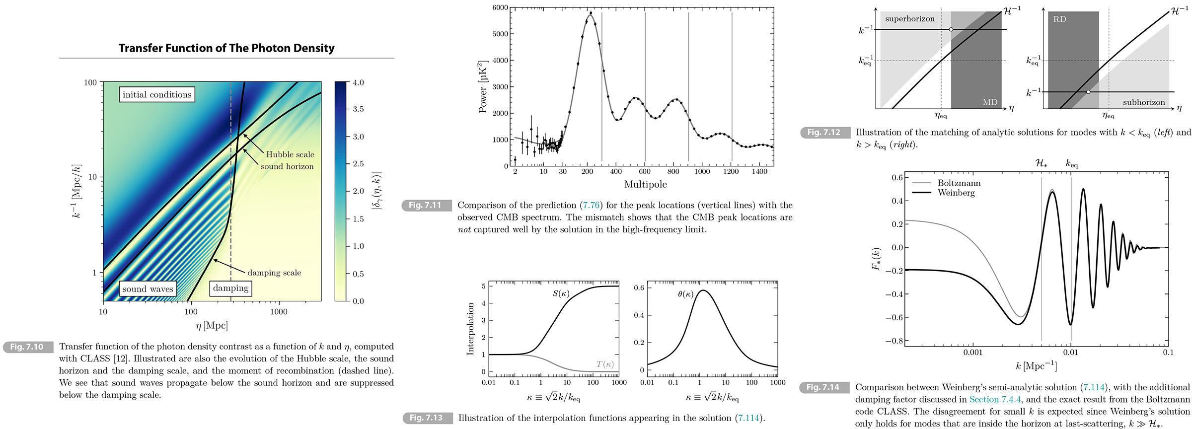
A numerical solution of the transfer function of the photon density contrast 𝛿𝛾 is shown in Fig. 7.10.
• Sound horizon Sound waves can only propagate if their wavelengths are smaller than the sound horizon
(7.54) 𝑟𝑠(𝜂) ≡ ∫𝜂0 d𝜂̄ 𝑐𝑠(𝜂̄),
where 𝑐𝑠 is the sound speed. [RE (5.11)] In Problem 7.2 we will show the comoving sound horizon at decoupling is 𝑟𝑠,* ≈ 135 Mpc. The effect of sound waves will only important for modes with 𝑘𝑟𝑠,* > 1. Since 𝑙 ~ 𝑘𝜒*, with 𝜒* ≈ 14 Gpc, this implies that sound waves should affect the CMB spectrum for 𝑙 > 100. This is indeed what is seen in the left panel of Fig. 7.7.
• Damping scale On small scales photon diffusion leads to a damping of the waves. High-energy photons in hot regions can diffuse into cold regions, thereby erasing the temperature difference. This diffusion can be modeled as a random walk, with the step size being photon's mean free path 𝓁𝛾 = 1/(𝑎𝑛𝑒𝜎𝛵). In a time interval ∆𝜂, the number of scattering is 𝛮 = ∆𝜂/𝓁𝛾 and the mean-squared distance explored by the random walk is ⟨∆𝑟2⟩ = 𝛮𝓁𝛾2 = 𝓁𝛾∆𝜂. Integrating this from 𝜂 = 0 to a time 𝜂, we get the squared diffusion length
(7.55) 𝑟𝐷2(𝜂) ~ ∫𝜂0 d𝜂̄ 𝓁𝛾(𝜂̄).
We see that the diffusion length is roughly the geometric mean between the age of the universe in conformal time and the mean free path of the photons. In Problem 7.3 we will show that the diffusion length at decoupling is 𝑟𝐷,* ≈ 7 Mpc. We will see in Section 7.4.4 that on scale smaller than the diffusion length, 𝑘𝑟𝐷,* > 1, the fluctuation are suppressed by a factor of 𝑒-2(𝑘𝑟𝐷,*)2. In harmonic space, the damping scale becomes 𝑙𝐷 ~ 𝜒*/√2𝑟𝐷,* ~ 1400, so we expect the CMB fluctuations to be exponentially damped for 𝑙 > 1400. In Section 7.4.4 we will improve this estimate.
7.4.1 Photon-Baryon Dynamics
Here we will re-derive the equations Thomson scattering does not exchange energy, so the the continuity equations for the photons and baryons still apply in their original forms [RE (5.14) (6.88) (6.85)]
Hydrodynamic equations
At linear order, the Thomson scattering does not exchange energy, so the continuity equations for the photons and baryons still apply in their original forms
(7.56) 𝛿𝛾ʹ = 4/3 𝑘𝑣𝛾 + 4𝛷ʹ,
(7.57) 𝛿𝑏ʹ = 𝑘𝑣𝑏 + 3𝛷ʹ.
Momentum on the other hand is exchanged by the scattering, so the Euler equations are modified. The Euler equation for photons becomes
(7.58) 𝑣𝛾ʹ + 1/4 𝑘𝛿𝛾 - 2/3 𝑘𝛱𝛾 + 𝑘𝛹 = -𝛤(𝑣𝛾 -𝑣𝑏),
where the source term on the right-hand side-called drag term-describes the momentum transfer between the photons and baryons. A formal derivation requires the Boltzmann equation and is given in Appendix B. The momentum transfer is proportional to the scattering rate, 𝛤, and to the difference between the photon and baryon velocities, 𝑣𝛾-𝑏 ≡ 𝑣𝛾 - 𝑣𝑏 (also called the slip velocity). Since the scattering tries to make the photons move together with baryons, so that 𝑣𝛾 → 𝑣𝑏 for large 𝛤. And the Euler equation for baryons is
(7.59) 𝑣𝑏ʹ + 𝓗𝑣𝑏 + 𝑘𝛹 = 𝛤/𝑅((𝑣𝛾 - 𝑣𝑏),
where the right-hand side is fixed by the requirement that the combined density must be conserved. The factor of 1/𝑅 simply arise because the baryons' momentum density is smaller than the photons' by a factor of 𝑅 ≡ 3/4 𝜌̄𝑏/𝜌̄𝛾. [RE (6.191)]
Tight-coupling limit
We first study these equations in the limit of large scattering rate. Let us begin by rearranging (7.59) as
(7.60) 𝑣𝛾-𝑏 = 𝑅/𝛤 [𝑣𝑏ʹ + 𝓗𝑣𝑏 + 𝑘𝛹].
To lowest order in 𝛤-1 the slip velocity is small, 𝑣𝛾-𝑏 ≈ 0. However, since 𝑣𝛾-𝑏 is multiplied by 𝛤 in the Euler equations, we need the next-to-leading order solution for it. We obtain this by substituting 𝑣𝑏 ≈ 𝑣𝛾, into the (7.60)
(7.61) 𝑣𝛾-𝑏 = 𝑅/𝛤 [𝑣𝛾ʹ + 𝓗𝑣𝛾 + 𝑘𝛹].
Using this in (7.58), we get
(7.62) 𝑣𝛾ʹ + 𝑅𝓗/(1 + 𝑅) 𝑣𝛾 + 1/4(1 + 𝑅) 𝑘𝛿𝛾 + 𝑘𝛹 = 0,
where we dropped the photon anisotropic stress 𝛱𝛾 which is suppressed for large 𝛤 (see below). Combining this with the continuity equation (7.56), we find a second-order equation for the photon density contrast
(7.63) 𝛿𝛾ʺ + 𝑅ʹ/(1+ 𝑅) 𝛿𝛾ʹ + 𝑘2𝑐𝑠2𝛿𝛾 = -3/4 𝑘2𝛹 + 4𝛷ʺ + 4𝑅ʹ/(1+ 𝑅) 𝛷ʹ,
where we used 𝑅𝓗 = 𝑅ʹ (since 𝑅 ∝𝑎) and introduce the sound speed 𝑐𝑠2 = [3(1 + 𝑅)]-1. [RE (6.198)] This is the same as (6.197) obtained in Section 6.4.
7.4.2 High-Frequency Solution
We will study to the solutions to master equation (7.63). We can make progress by studying special limits. We first consider the high-frequency limits, 𝑘 ≫ 𝓗. Following Weinberg [Weinberg], we split the solution into "fast" and "slow" modes
(7.64) 𝑓 = 𝑓fast + 𝑓slow,
where 𝑓 ≡ {𝛿𝛾, 𝛹, 𝛷). The fast modes evolve on a scale 𝑘-1, so that ∂𝜂𝑓fast ~ 𝑘𝑓fast, while the slow modes vary on the Hubble time scale 𝓗-1, so that ∂𝜂𝑓slow ~ 𝓗𝑓slow. Dark matter fluctuations do not have any fast modes (because the dark matter is pressureless). The fast modes of the gravitational potential is sourced by the radiation fluctuations. From the Poisson equation, we have
(7.65) -𝑘2𝛷fast = 4π𝐺𝑎2𝜌̄𝛾𝛿𝛾fast ≲ 𝓗2𝛿𝛾fast,
so that the gravitational potential 𝛷fast is suppressed by a factor of 𝓗2/𝑘2 ≪ 1 in the high-frequency limits. The fast mode of the photon density contrast obeys the homogeneous equation
(7.66) 𝛿𝛾ʺ + 𝑅ʹ/(1+ 𝑅) 𝛿𝛾ʹ + 𝑘2𝑐𝑠2𝛿𝛾 = 0 (fast mode).
This equation can be solved in a WKB approximation (see Problem 7.4). Consider the ansatz
(7.67) 𝛿𝛾 = 𝛢(𝜂)exp[±𝑖𝑘 ∫𝜂0 𝑐𝑠(𝜂̄) d𝜂̄] ≡ 𝛢(𝜂)𝑒±𝑖𝜑(𝜂),
where the function 𝛢(𝜂) is slowly varying on the timescale of the oscillations. Taking time derivatives of (7.67). we get
(7.68) 𝛿𝛾ʹ = 𝛢ʹ𝑒±𝑖𝜑 ± 𝑖𝑘𝑐𝑠𝛢𝑒±𝑖𝜑 ≈ 𝑖𝑘𝑐𝑠𝛿𝛾,
(7.69) 𝛿𝛾ʺ = 𝛢ʹ𝑒±𝑖𝜑 ± 2𝑖𝑘𝑐𝑠𝛢ʹ𝑒±𝑖𝜑 ± 𝑖𝑘𝑐𝑠ʹ𝛢𝑒𝑖𝜑 - 𝑘2𝑐𝑠2𝛢𝑒𝑖𝜑 ≈ [± 2𝑖𝑘𝑐𝑠𝛢ʹ/𝛢 ∓ 𝑖𝑘𝑐𝑠/2 𝑅ʹ/(1+ 𝑅) - 𝑘2𝑐𝑠2]𝛿𝛾,
where we used 𝛢ʹ ≪ 𝑖𝑘𝑐𝑠𝛢, 𝛢ʺ ≪ 𝑖𝑘𝑐𝑠𝛢ʹ and
(7.70) 𝑐𝑠ʹ = d/d𝜂 [1/√3(1 + 𝑅)] = -1/2 𝑐𝑠 𝑅ʹ/(1+ 𝑅).
Substituting (7.68) and (7.69) into (7.66) then gives
(7.71) 𝛢ʹ/𝛢 = -1/4 𝑅ʹ/(1+ 𝑅) ⇒ 𝛢(𝜂) ∝(1 + 𝑅)-1/4, [taking the derivative of logarithm of both sides]
and the solution of (7.66) takes the form
(7.72) 𝛿𝛾fast = (1 + 𝑅)-1/4[𝐶 cos(𝜑) + 𝐷 sin(𝜑)].
The integration constants 𝐶 and 𝐷 are fixed by the superhorizon initial conditions. For adiabatic initial conditions, we expect 𝐶 ≫ 𝐷 and oscillating part of the solution is a pure cosine.
To complete the solution we must add the slow mode of the photon density contrast. In this case we can drop all time derivative terms in (7.63) and the solution becomes
(7.73) 𝛿𝛾slow = -4(1 + 𝑅)𝜓slow,
where 𝜓slow is now also sourced by the dark matter perturbations. The full WKB solution is
(7.74) 𝛿𝛾 = (1 + 𝑅)-1/4[𝐶 cos(𝜑) + 𝐷 sin(𝜑)] - 4(1 + 𝑅)𝜓.
We see that the gravitational force term has shifted the zero-point of the oscillations. Since the gravitational potential decays on sub-Hubble scales during the radiation era, the size of the zero-point shift will depend on the time that the mode has spent inside the horizon during the era (which is dedicated by the wavelength of the fluctuation).
The transfer function for the Sachs-Wolfe term is
(7.75) 𝐹*(𝑘) = 1/4 𝛿𝛾(𝜂*, 𝐤) + 𝛹(𝜂*, 𝐤) = 1/4 (1 + 𝑅)-1/4[𝐶 cos(𝜑*) + 𝐷 sin(𝜑*)]/𝓡𝑖(𝐤) - 𝑅 𝛹(𝜂*, 𝐤)/𝓡𝑖(𝐤), [RE (6.55) (6.150) (6.155) (6.165) (7.31) (7.44)]
with 𝜑* = 𝑘𝑟𝑠,*. In Section 7.3.3 we saw that the angular power spectrum is given roughly by ∣𝐹*(𝑘)∣2, with 𝑘 ≈ 𝑙/𝜒*. Since 𝐶 ≫ 𝐷, we expect the peaks of the spectrum to be at [RE (7.3), p 267, (7.49)]
(7.76) 𝑙𝑛 = 𝑛π 𝜒*/𝑟𝑠,* ≈ 𝑛π (14 Gpc)/(145 Mpc) ≈ 𝑛 × 302,
where 𝑛 ∊ 𝐙(interger). However the prediction does not match the measured locations of the first few peaks, 𝑙1 = 220.0±0.5, 𝑙2 = 537.5±0.7 and 𝑙2 = 810.8±0.7 [11]. A graphical illustration of this mismatch is given in Fig. 7.11. While the prediction (7.76) works well for the peak spacing, the predicted peak locations is shifted by about one fourth of the oscillation period here.
7.4.3 Semi-Analytic Solution*
There is no analytic solution for the dynamics of the photon-baryon fluid valid at all times and for all wavelengths. However Weinberg found an good semi-analytic solution using interpolation between two analytic solution for 𝑘 ≪ 𝑘eq and 𝑘 ≫ 𝑘eq. The following is a summary [Weinberg]. An alternative solution by Hu and Sugiyama [12] is discussed in Problem 7.5.
• Modes with 𝑘 < 𝑘eq are outside the horizon during the radiation era and enter the horizon during the matter era. The superhorizon evolution of the fluctuations is known analytically. In the matter era an analytic solution is possible on all scales. By matching this to the superhorizon solution we obtain an analytic solution for 𝑘 < 𝑘eq (see Fig. 7.12). For realistic parameters, the time of decoupling 𝜂* relatively close to 𝜂eq, assuming 𝜂* ≫ 𝜂eq is still useful because it motivates an ansaz for the interpolation function, which will apply at 𝜂*.
• Modes with 𝑘 > 𝑘eq instead enter the horizon during the radiation era. In the radiation era an analytic solution exists for all 𝑘. Once the mode is deep inside the horizon, an analytic solution is possible that remains valid when matter becomes important. By matching the two solutions in the region of overlap-i.e. for subhorizon modes in the radiation era-we obtain an analytic solution for 𝑘 > 𝑘eq with yhe correct initial conditions (see Fig. 7.12).
The two analytic solutions will first be derived and then Weinberg's interpolation will be described.
Long-wavelength solution
We first consider modes with 𝑘 < 𝑘eq. They are derived in Section 6.2 and Problem 6.1. There we found that the superhorizon limit of the photon density contrast in the matter era is
(7.77) 𝛿𝛾 = 4/3 𝛿𝑐 = -8/3 𝛷 (𝑘 < 𝓗 < 𝑘eq),
where we used that 𝛿𝑐 = -2𝛷. In terms of the curvature perturbation 𝓡𝑖(𝐤), we have [RE (6.150) (6.155)]
(7.78) 𝛹 ≈ 𝛷 = 3/5 𝓡𝑖, 𝛿𝛾 = -8/5 𝓡𝑖 (𝑘 < 𝓗 < 𝑘eq).
We will use this as an initial condition for the modes entering the horizon during the matter era.
Initially the effect of baryon is still negligible, 𝑅 ≪ 1, [RE (6.191)] and the (7.63) becomes
(7.79) 𝛿𝛾ʺ + 1/3 𝑘2𝛿𝛾 = -4/3 𝑘2𝛹,
where we used that 𝛷 is a constant during the matter era. This equation is valid on all scales. Its solution is
(7.80) 𝛿𝛾 = 𝐶 cos(𝜑) + 𝐷 sin(𝜑) - 4𝛹,
where 𝜑 = 𝑘𝜂/√3. Matching the 𝜑 ≪ 1 limit of (7.80) to the superhorizon limit (7.78), we get
(7.81) 𝛿𝛾 = 4/5 𝓡𝑖[cos(𝜑) - 3].
Eventually 𝑅 becomes large and with 𝑘 > 𝓗 this happens when they are already deep inside the horizon. Then the WKB solution (7.74) applies and we have
(7.82) 𝛿𝛾 = 4/5 𝓡𝑖[(1 + 𝑅)-1/4 cos(𝜑) - 3(1 + 𝑅)] (𝑘 < 𝑘eq),
where 𝜑 = 𝑘 ∫ d𝜂/√3(1 + 𝑅). This solution is smoothly connected to the solution in (7.81).
Short-wavelength solution
Next, we consider modes with 𝑘 > 𝑘eq. which entered the Hubble radius during the radiation era. We first derive an analytic solution in the radiation era and then mach its the high-frequency limit to WKB solution (7.74).
During the radiation era with 𝑅 ≪ 1 and the effects of the baryons can be ignored. This simplifies the (7.63) to
(7.83) 𝛿𝛾ʺ + 1/3 𝑘2𝛿𝛾 = -4/3 𝑘2𝛹 + 4𝛷ʺ,
where the time dependence of metric potentials must now be account for. Defining 𝑑𝛾 ≡ 𝛿𝛾 - 4𝛷 [RE (6.127)] and 𝜑 = 𝑘𝜂/√3, we get
(7.84) 𝑑𝛾ʺ + 𝑑𝛾 = -4(𝛷 + 𝛹),
where the prime is for a derivative respect to 𝜑. The solution is
(7.85) 𝑑𝛾 = 𝐶 cos(𝜑) + 𝐷 sin(𝜑) - 4∫𝜑0 d𝜑̂ sin(𝜑 - 𝜑̂) (𝛷 + 𝛹)(𝜑̂),
where 𝐶 = -4𝓡𝑖 and 𝐷 = 0 for adiabatic initial conditions.
Exercise 7.4 Let 𝑆1 = cos(𝜑) and 𝑆2 = sin(𝜑) be the two homogeneous solutions of (7.84). Using
(7.86) 𝐺(𝜑, 𝜑̂) = [𝑆1(𝜑̂)𝑆2(𝜑) - 𝑆1(𝜑)𝑆2(𝜑̂)]/[𝑆1(𝜑)𝑆2ʹ(𝜑) - 𝑆1ʹ(𝜑)𝑆2(𝜑)],
confirm the form of the Green's function in (7.85).
[Solution] 𝐺(𝜑, 𝜑̂) = [cos(𝜑̂)sin(𝜑) - cos(𝜑)sin(𝜑̂)]/[cos2(𝜑) + sin2(𝜑)] = cos(𝜑̂)sin(𝜑) - cos(𝜑)sin(𝜑̂) = sin(𝜑 - 𝜑̂). ▮
Using the relation sin(𝜑 - 𝜑̂) = sin(𝜑)cos(𝜑̂) - cos(𝜑)sin(𝜑̂), (7.85) can be written as
(7.87) 𝑑𝛾 = (𝐶 + ∆𝐶) cos(𝜑) + ∆𝐷 sin(𝜑),
(7.88-9) ∆𝐶 = 4∫𝜑0 d𝜑̂ sin(𝜑̂) (𝛷 + 𝛹)(𝜑̂), ∆𝐷 = -4∫𝜑0 d𝜑̂ cos(𝜑̂) (𝛷 + 𝛹)(𝜑̂).
To evaluate this we need the solutions for 𝛷(𝜂) and 𝛹(𝜂), which were found in Section 6.3.1. Ignoring the anisotropic stress due to neutrinos, we obtained [RE (6.165)]
(7.90) 𝛷 = 𝛹 = 2𝓡𝑖 [sin(𝜑) - 𝜑 cos(𝜑)]/𝜑3.
Substituting this into (7.88) and (7.89), we get
(7.91-2) ∆𝐶 = 8𝓡𝑖 [1- sin2(𝜑)/𝜑2], ∆𝐷 = 8𝓡𝑖 [cos(𝜑) sin(𝜑) - 𝜑]/𝜑2,
and (7.87) becomes
(7.93) 𝑑𝛾 = 4𝓡𝑖 [cos(𝜑) - 2sin(𝜑)/𝜑].
This is a remarkably simple solution for the fluctuations in the radiation era, valid on all scales. The solution is only a pure cosine curve in the high-frequency limits, 𝜑 ≫ 1. For intermediate wavelengths the gravitational evolution has led to an admixture.
To extend this into the matter era, we match the 𝜑 ≫ 1 limit of (7.93), 𝑑𝛾 → 𝛿𝛾 ≈ 4𝓡𝑖cos(𝜑) to the WKB solution (7.74). The resulting solution is
(7.94) 𝛿𝛾 = 4𝓡𝑖(1 + 𝑅)-1/4 cos(𝜑) - 4(1 + 𝑅)𝛹.
To complete the analysis we need to relate 𝛹 to 𝓡𝑖. in the matter era, we have [RE (6.53) (6.134)]
(7.95) 𝛹 ≈ 3/2 𝓗2/𝑘2 𝛿𝑐,
so 𝛹 can be obtained from the solution for the dark matter density contrast 𝛿𝑐. It will be shown below (7.98)
(7.96-7) 𝛿𝑐 ≈ -1.54𝓡𝑖 ln (0.15 𝑘/𝑘eq)(𝑘eq 𝜂)2 (𝑘 > 𝑘eq); 𝛹 ≈ 3/5 𝓡𝑖 ln(0.15 𝑘/𝑘eq)/(0.31 𝑘/𝑘eq)2.
Feeding this into (7.94), we obtain the solution for the photon density contrast in the matter era:
(7.98) 𝛿𝛾 = 4/5 𝓡𝑖[5(1 + 𝑅)-1/4 cos(𝜑) - 3(1 + 𝑅) ln(0.15 𝑘/𝑘eq)/(0.31 𝑘/𝑘eq)2] (𝑘 > 𝑘eq).
Compared to the long-wavelength solution (7.82), he amplitude is enhanced by a factor of 5 and the zero-point is shfted by a nontrivial transfer function.
Derivation In the following we derive the dark matter transfer function for 𝑘 > 𝑘eq. The continiuty and Euler equations for dark matter are [RE (6.85-6)]
(7.99-100) 𝛿𝑐ʹ = 𝑘𝑣𝑐 + 3𝛷ʹ, 𝑣𝑐ʹ + 𝓗𝑣𝑐 = -𝑘𝛹.
Substituting (7.99) into (7.100) and defining 𝑑𝑐 ≡ 𝛿𝑐 - 3𝛹,
(7.101) (𝑎𝑑𝑐ʹ)ʹ = -3𝑎𝛹, [verification needed]
where primes denote derivatives with respect to 𝜑 ≡ 𝑘𝜂/√3, Integrating (7.101), we get
(7.102) 𝑑𝑐(𝜑) = -3∫𝜑0 d𝜑̂/𝑎 ∫𝜑̂0 𝑎𝛹(𝜑̄) d𝜑̄.
This result is exact and valid for all 𝑘. During the radiation era the gravitational potential is determined by the radiation and 𝛹 can be treated as an external source as far as the evolution of dark matter is concerned. We can use (7.90) and 𝑎 ∝ 𝜂 ∝ 𝜑 to evaluate the integral
(7.103) 𝑑𝑐(𝜑) = -3∫𝜑0 d𝜑̂/𝜑̂ ∫𝜑̂0 𝑎𝛹(𝜑̄) d𝜑̄ = -6𝓡𝑖∫𝜑0 d𝜑̂/𝜑̂ ∫𝜑̂0 [sin(𝜑̄) - 𝜑̄ cos(𝜑̄)]/𝜑̄2 d𝜑̄ = -6𝓡𝑖∫𝜑0 d𝜑̂/𝜑̂ [1 - sin(𝜑̂)/𝜑̂] + 𝑑𝑐(0),
where the integration constant is fixed by the superhorizon limit, 𝑑𝑐(0) = -3𝓡𝑖. [verification needed] Solving the integration, we find [using WolframAlpha]
(7.104) 𝑑𝑐(𝜑) = 6𝓡𝑖[Ci(𝜑) - sin(𝜑)/𝜑 - ln 𝜑]∣𝜑0 - 3𝓡𝑖,
where Ci(𝜑) is the cosine integral
(7.105) Ci(𝜑) ≡ -∫∞𝜑 cos(𝜑̂)/𝜑̂ d𝜑̂. [added '-' unlike the text; RE Wikipedia Trigonometric integral]
The superhorizon limit of the cosine integral is
(7.106) lim𝜑→0 Ci(𝜑) = 𝛾𝐸 + ln 𝜑 - 𝑂(𝜑2), [RE 𝑂(𝜑2) = 𝜑2/4]
where 𝛾𝐸 = 0.5772 ... is the Euler-Mascheroni constant, while the high-frequency limit, 𝜑 → ∞, vanishies by definition.
(7.107) 𝑑𝑐(𝜑) →𝜑≫1 𝑑𝑐(𝜑) = 6𝓡𝑖[1/2 - 𝛾𝐸 - ln 𝜑 + 𝑂(𝜑-1)], [verification needed]
which describes the evolution after the mode entered the horizon but before matter-radiation equality.
We would like to compare this solution to the solution (6.181) for matter fluctuation on sub-Hubble scales (but not restricted to the radiation era):
(7.108) 𝛿𝑐 = 𝐶1(1 + 3/2 𝑦) + 𝐶2[(1 + 3/2 𝑦) ln[{√(1 + 𝑦) + 1}/{√(1 + 𝑦) - 1}] - 3√(1 + 𝑦)].
where 𝑦 ≡ 𝑎/𝑎eq. In the limit 𝑦 ≪ 1, this solution gives
(7.109) 𝛿𝑐 →𝑦≪1 (𝐶1 -3𝐶2) - 𝐶2 ln(𝑦/4) + 𝑂(𝑦) = [𝐶1 -3𝐶2) - 𝐶2 ln[2/√3(√2 - 1) 𝑘/𝑘eq]] - 𝐶2 ln 𝜑, [verification needed]
where we used (2.162) to relate 𝑦 ∝ 𝜂 to 𝜑 [= 𝑘𝜂/√3] and introduced 𝑘eq = 𝜂eq-1. This is consistent with (7.107) if
(7.110) 𝐶1 = 6𝓡𝑖 [7/2 - 𝛾𝐸 - ln[2/√3(√2 - 1) 𝑘/𝑘eq]] ≈ -6𝓡𝑖 ln(0.15 𝑘/𝑘eq). [verification needed]
(7.111) 𝐶2 = 6𝓡𝑖.
During the matter-dominate era (𝑦 ≫ 1), the second term in (7.108) is a decaying mode and can be dropped. We then find
(7.112) 𝛿𝑐 →𝑦≫1 3/2 𝐶1𝑦 = -9𝓡𝑖 ln(0.15 𝑘/𝑘eq) (𝑘eq𝜂)2(√2 - 1)2 ≈ -1.54𝓡𝑖 ln(0.15 𝑘/𝑘eq) (𝑘eq𝜂)2,
where we used (2.162) for 𝑦 ∝ 𝜂2 in the matter era. This solution has the ln 𝑘 scaling that we found in Section 6.3.2, but now includes the precise numerical factors that are required to relate 𝛿𝑐 to 𝓡𝑖.
Solution at last-scattering
The analytic solutions (7.82) and (7.98) imply the following limits of Sachs-Wolfe transfer function at last-scattering:
(7.113) 𝐹*(𝑘) ≡ (1/4 𝛿𝛾 + 𝛹)*/𝓡𝑖 [RE 7.31)]
= { 1/5 [1/(1 + 𝑅*)1/4 cos(𝑘𝑟𝑠,*) - 3𝑅*] 𝑘 < 𝑘eq; 1/5 [5/(1 + 𝑅*)1/4 cos(𝑘𝑟𝑠,*) - 3𝑅* ln(0.15𝑘/𝑘eq)/(0.31𝑘/𝑘eq)2] 𝑘 > 𝑘eq
We would like to find a solution that interpolates between these two limits valid with 𝑘 ~ 𝑘eq. Motivated by the solutions in (7.113), Weinberg proposed the following ansatz
(7.114) 𝐹*(𝑘) = 1/5 [𝑆(𝑘)/(1 + 𝑅*)1/4 cos[𝑘𝑟𝑠,* + 𝜃(𝑘)] - 3𝑅*𝛵(𝑘)],
with 𝛵(𝑘), 𝑆(𝑘) and 𝜃(𝑘) are momentum-dependent interpolation functions, with limits
(7.115) 𝑘 ≪ 𝑘eq: 𝑆 → 1, 𝛵 → 1, 𝜃 → 1,
𝑘 ≫ 𝑘eq: 𝑆 → 5, 𝛵 → ln(0.15𝑘/𝑘eq)/(0.31𝑘/𝑘eq)2, 𝜃 → 0,
The interpolation between 𝑘 ≪ 𝑘eq and 𝑘 ≫ 𝑘eq can almost be done "by hand," with reasonable results for the CMB spectrum. The result is summarized by the following fitting functions [Weinberg]
(7.116) 𝑆(𝜅) ≡ [[1 + (1.209𝜅)2 + (0.5116𝜅)4 + √5(0.1657𝜅)6]/[1 + (0.9459𝜅)2 + (0.249𝜅)4 + √(0.167𝜅)6]]2,
𝛵(𝜅) ≡ [ln[1 + (0.124𝜅)2]/(0.124𝜅)2 [[1 + (1.257𝜅)2 + (0.4452𝜅)4 + (0.2197𝜅)6]/[1 + (1.606𝜅)2 + (0.8568𝜅)4 + (0.3927𝜅)6]]1/2,
𝜃(𝜅) ≡ [[(1.1547𝜅)2 + (0.5986𝜅)4 + (0.2578𝜅)6]/[1 + (1.723𝜅)2 + (0.8707𝜅)4 + (0.458𝜅)6 + (0.2204𝜅)8]]1/2,
where 𝜅 ≡ √2𝑘/𝑘eq. Plots of these fitting functions are given in Fig. 7.13. Note that it takes quite long for these functions to reach the high-frequency limit, especially 𝑆(𝜅).
The function 𝜃(𝜅) leads to shifts in the CMB peak positions relative to the high-frequency solution in Section 7.4.1.7 As Weinberg showed, the agreement with the observed peak positions is now "almost embarrassingly good" [Weinberg]. Indeed Weinberg's SW transfer function (7.114) shows perfect agreement of the oscillatoty part with the exact numerical result in Fig. 7.14. The disagreement at small 𝑘 is expected since Weinberg's solution only applies to subhorizon modes at last-scattering. In this low-frequency limit, we should take 𝑅* → 0 in (7.114) since sound waves are not important on these large scales. This reproduce the correct SW limit of Section 7.3.2.
The solution above does not contain the effects of neutrinos. The neutrinos's anisotropic stress on the superhorizon initial conditions for metric potential is small as we see in Problem 6.2. The free-straming neutrinos leads to a small phase shift in the high -frequency limit of the solution [13, 14], 𝜃(𝑘 ≫ 𝑘eq) → 0.063π. These effects have to be considered to match the precision of current experiments, but are't essential for understanding the main feature of the CMB spectrum.
From the solution for photon density contrast, we can infer the baryon velocity and hence the transfer functon for the Doppler contribution. Using the continuity equation for photon during the matter era reads 𝛿𝛾ʹ 4/3 𝑘𝑣𝛾, we obtain 𝐺*(𝑘) = (𝑣𝑏)*/𝓡𝑖 ≈ (𝑣𝛾)*/𝓡𝑖 = 3(𝛿𝛾ʹ)*/(4𝓡𝑖𝑘). Taking the derivative of the solution for 𝛿𝛾 with respect to conformal tme, we find
(7.117) 𝐺*(𝑘) = -√3/5 𝑆(𝑘)/(1 + 𝑅*)3/4 sin[𝑘𝑟𝑠,* + 𝜃(𝑘)].
We see that the oscillations in the Doppler term are exactly out of phase with those in the photon density.
7.4.4 Small-Scaling Damping
We saw in the plots of the CMB spectrum that the ower is suppressed for multipoles (𝑙 > 1000). This damping is nnotyet included. There are two sources of damping: First, photon deiffusion between hot and cold regions erases tempurature differences on small scales. Second, the surface of last-scattering has a finite thickness. Averaging over this finite width suppresses short-wavelength fluctuations. We will derive these two effects.
Silk damping
since the effect of photon diffusion is only important deep inside the Hubble radius, we can ignore the effects of expansion: e.g. 𝓗𝑣𝑏 ≪ 𝑣𝑏ʹ in the Euler equation (7.59). We can also drop the gravitational forcing terms, since -𝑘2𝛷 ~ 𝓗2𝛿, so that 𝑘𝛹 is small relative to the photon pressure term, 𝑘𝛿𝛾, and the change in the baryon momentum density, 𝑅𝑣𝑏ʹ. The Euler equations are
(7.118-9) 𝑣𝛾ʹ + 1/4 𝑘𝛿𝛾 - 2/3 𝑘𝛱𝛾 = -𝛤𝑣𝛾-𝑏, 𝑅𝑣𝑏ʹ = +𝛤𝑣𝛾-𝑏,
we restored the photon anisotropic stress 𝛱𝛾. Above we studied these equations at leading order in an expansion in 𝑘/𝛤 = 𝑘𝓁𝛾 < 1. [verification needed] We will extend the treatment to include the next-to-leading order correction capturing the damping fluctuations. Combining the two Euler equations, we get the slip velocity equation
(7.120) 𝑣ʹ𝛾-𝑏 = - (1 + 𝑅)/𝑅 𝛤𝑣𝛾-𝑏 - 1/4 𝑘𝛿𝛾 + 2/3 𝑘𝛱𝛾.
In the tight-coupling limit we can drop the photon anisotropic stress and the time variation of the slip velocity. We then have
(7.121) 𝑣𝛾-𝑏 ≈ - 𝑅/(1 + 𝑅) 𝑘/𝛤 𝛿𝛾/4.
his equation has an interesting physical interpretation: the slip velocity characterizes the bulk velocity of the photons in the rest frame of the baryons and is therefore associated with an energy flux in that frame. Since 𝜌𝛾 ∝ 𝛵𝛾4, the right-hand side of (7.121) can be written as -𝓁𝛾𝛁𝛵𝛾/𝛵̄, which means That it describes the energy flux coming from a gradient in the photon temperature. A finite slip velocity is therefore associated with thermal conduction.
Adding the two Euler equations, we find
(7.122) 𝑅𝑣𝑏ʹ + 𝑣𝛾ʹ + 1/4 𝑘𝛿𝛾 - 2/3 𝑘𝛱𝛾 = 0.
Using the conduction equation (7.121), the time derivative of the baryon velocity can be written as
(7.123) 𝑣𝑏ʹ = 𝑣𝛾ʹ - 𝑣ʹ𝛾-𝑏 ≈ 𝑣𝛾ʹ + 𝑅/(1 + 𝑅) 𝑘/𝛤 𝛿𝛾ʹ/4,
where we ignored time derivatives of 𝑅 and 𝛤 on sub-Hubble scales. Equation (7.122) becomes
(7.124) (1 + 𝑅)𝑣𝛾ʹ = -1/4 𝑘𝛿𝛾 - 𝑅2/4(1 + 𝑅) 𝑘/𝛤 𝛿𝛾ʹ + 2/3 𝑘𝛱𝛾.
In Appendix B, we show that the photon anisotropic stress is related to the gradient of the bulk velocity (see section B.3.1)
(7.125) 𝛱𝛾 ≈ -4/9 𝑘/𝛤 𝑣𝛾,
which leads t an effective photon viscosity. Equation (7.124) reads [RE Wikipedia Viscosity - the first term in the right-hand side]
(7.126) (1 + 𝑅)𝑣𝛾ʹ = -1/4 𝑘𝛿𝛾 - 1/4 [8/9 + 𝑅2/(1 + 𝑅)] 𝑘/𝛤 𝛿𝛾ʹ,
where we used the continuity equation on sub-Hubble scales, 𝛿𝛾ʹ = 4/3 𝑘𝑣𝛾. [RE (6.88)] Taking a time derivative of the continuity equation, 𝛿𝛾ʺ = 4/3 𝑘𝑣𝛾ʹ, and substituting (7.126) hen gives
(7.127) 𝛿𝛾ʺ + 𝑘2/3(1 + 𝑅) 1/𝛤 [8/9 + 𝑅2/(1 + 𝑅)]𝛿𝛾ʹ + 𝑘2𝑐𝑠2 𝛿𝛾 = 0.
We see that going beyond leading order in the tight-coupling approximation has introduced a friction term to 𝛿𝛾ʹ. This friction is a combination of thermal conduction and photon viscosity. The size of the friction term depends on the wavenumber 𝑘. The associated damping of the fluctuations is called Silk damping [15].
We can solve (7.127) in a WKB approximation. Consider the ansatz
(7.128) 𝛿𝛾 ∝ exp[𝑖∫𝜂0 𝜔(𝜂') d𝜂'], with 𝜔ʹ ≪ 𝜔2.
Taking time derivatives of it, we get
(7.129) 𝛿𝛾ʹ = 𝑖𝜔𝛿𝛾
(7.130) 𝛿𝛾ʺ = (-𝜔2 + 𝑖𝜔ʹ)𝛿𝛾 ≈ -𝜔2𝛿𝛾,
and using this in (7.127), we find
(7.131) (𝑘2𝑐𝑠2 - 𝜔2) + 𝑘2/3(1 + 𝑅) 1/𝛤 [8/9 + 𝑅2/(1 + 𝑅)]𝑖𝜔 = 0.
Substituting 𝜔 = 𝑘𝑐𝑠 + 𝛿𝜔, and expanding in small 𝛿𝜔, gives
(7.132) 𝛿𝜔 = 𝑖𝑘2/6(1 + 𝑅) 1/𝛤 [8/9 + 𝑅2/(1 + 𝑅)]
[Derivation 𝑘2𝑐𝑠2 - 𝜔2 + 2𝛿𝜔 = 0. ⇒ 𝜔 = 1/2 ±√(4𝑘𝑐𝑠2 - 2𝛿2) + ≈ 𝑘𝑐𝑠 + 𝛿𝜔. ▮]
Since the correction is imaginary, the solution (7.128) receives an exponential suppression
(7.133) 𝛿𝛾 ∝ 𝑒-𝑘2/𝑘𝑆2 exp[𝑖𝑘 ∫ 𝑐𝑠(𝜂') d𝜂'],
where the damping wavenumber is
(7.134) 𝑘𝑆-2(𝜂) ≡ ∫𝜂0 d𝜂'/[6(1 + 𝑅)𝛤(𝜂') [8/9 + 𝑅2/(1 + 𝑅)].
Including polarization corrections to the scattering would give the same result with 8/9 → 16/15 [16]. We see that diffusion damping can be modeled by an 𝑒-𝑘2/𝑘𝑆2 envelope to the oscillatory part in the previous section. Therefore this replaces the transfer function 𝑆(𝑘) in Weinberg's solutions (7.114) and (7.117) with 𝑒-𝑘2/𝑘𝑆,*2𝑆(𝑘) where 𝑘𝑆,* is given by (7.134) evaluated at last-scattering. For standard cosmological parameters, a good estimate of the Silk damping scale is (see Problem 7.3)
(7.135) 𝑘𝑆,*-1 ≈ 7.2 Mpc.
This corresponds to damping in the CMB power spectrum for multipoles larger than 𝑙𝑆 ~ 𝑘𝑆,*𝜒*/√2 ~ 1370.[verification needed]
Landau damping
So far we have assumed that recombination was an instantaneous process,, corresponding to the visibility function being a perfect delta function. But as we see from Fig. 7.5 , in reality it has a finite width. For short-wavelength fluctuations this has to be taken into account.
Near its maximum, the visiblity function can be approximated by a Gaussian
(7.136) 𝑔(𝜂) = exp[-(𝜂 - 𝜂*)2/3𝜎𝑔2]/√(2π)𝜎𝑔,
where 𝜎𝑔 ≈ 15.5 Mpc. The fluctuations must now be averaged over this finite width of the function. This averaging makes little difference for slowly evolving fluctuations which can be enhanced at the mean time of decoupling 𝜂*. The amplitude of the rapidly oscillating part can be significantly reduced by averaging. This effect is called Landau damping because it is similar to the damping that occurs for oscillations with a spread frequencies.
In Appendix B we derive the line-of-sight solution in the visibility function; see Section B.2. For Sachs-Wolfe term, we find
(7.137) 𝛳SW𝑙(𝑘) = ∫𝜂00 d𝜂 𝑔(𝜂) (1/4 𝛿𝛾 + 𝛹) 𝑗𝑖(𝑘𝜒),
where 𝜒(𝜂) = 𝜂 - 𝜂*. Over the small range of support of the visibility function, the Bessel function can be time independent and be pulled out of the integral. The remaining integral is
(7.138) ∫𝜂00 d𝜂 𝑔(𝜂) cos[∫𝜂0 𝜔(𝜂') d𝜂'] ≈ ∫𝜂00 d𝜂 𝑔(𝜂) cos[∫𝜂*0 𝜔(𝜂') d𝜂' + 𝜔*(𝜂 - 𝜂*)] ≈ exp(-𝜔*2𝜎𝑔2/2) cos[∫𝜂*0 𝜔(𝜂') d𝜂'],
where 𝜔* = 𝜔(𝜂*) = 𝑘𝑐𝑠,*. We see that the averaging induced an exponential damping factor exp(-𝑘2/𝑘𝐿,*2), with a scale
(7.139) 𝑘𝐿,*-1 = 𝑐𝑠,*𝜎𝑔/√2 = 𝜎𝑔/√(6(1 + 𝑅*) ≈ 5.0 Mpc.
Since the functional dependence of this effect is the same as for Silk damping, we can combine the two. To obtain the effective damping scale, the two damping scales must be added in quadrature
(7.140) 𝑘𝐷,*-1 = √(𝑘𝑆,*-2 + 𝑘𝐿,*-2) ≈ 8.8 Mpc.
The multiple mement corresponding to this damping scale is 𝑙𝐷 ~ 𝑘𝐷,*𝜒*/√2 ~ 1125, which agrees with the observed CMB spectrum in Fig. 7.2.
7 The phase shift analytically is possible but quite nontrivial. The phase shift 𝜃(𝜅) has multiple origins, such as the breakdown of tight coupling, neutrino free-streaming and a transient of gravitational potential. Moreover the significant part of mismatch in the predicted peak locations (7.76) comes from that the 𝑙 ~ 𝑘𝜒* mapping is not very accurate [11]and this account for about half of the shifts seen in Fig. 7.11 and the rest is captured by the nontrivial phase shift 𝜃(𝜅). |
|
|