|
김관석
|
2024-09-27 11:10:45, 조회수 : 88 |
- Download #1 : BC_4a.jpg (412.9 KB), Download : 0

4 Cosmological Inflation
The standard BB theory described in the previous two chapters is incomplete. Key features of the observed universe, such as its large-scale homogeneity and flatness, seem to require that the universe started with very special, finely tuned initial conditions. These initial conditions must be imposed by hand. In this chapter, how inflation-an early period of accelerated expansion-drives the primordial universe towards the special state, even if it started from more generic initial conditions.
To specify the initial condition, we define the position and velocities of all particles on an initial time slice, or in the fluid approximation, we specify the density and pressure as a function of position. The laws of gravity and fluid dynamics are then used to evolve the system forward in time. We assumed the distribution of matter to be homogeneous and isotropic. But, why is this good assumption? How do we explain the extraordinary smoothness of the early universe? This is particularly surprising since most of universe appears not be have been in causal contact and there is no dynamical reason why these causally-disconnected regions have such similar physical properties. This homogeneity problem is often called horizon problem.
Additionally in order for the universe to remain homogeneous at late times the initial fluid velocities must take very precise value. If the initial velocities are just slightly small, the universe recollapses within a fraction of a second. If they are just slightly too big, the universe expands too rapidly and quickly becomes nearly empty. The fine-tuning of the initial velocities is made even more dramatic by considering it in the combination with the horizon problem, since the fluid velocities need to be fine-tuned across causally-disconnected regions of space. In Section 2.3.5, we see that local curvature of a region in space is determined by the sum of the particles and kinetic energies in that region. The fine-tuning of the initial velocities is therefore often called the flatness problem and can be phrased as the question why the spatial curvature of the universe is so small.
Maybe it could be argued on the basis of symmetry that perfect homogeneity and exact flatness are preferred set of initial conditions and appeal to an unknown theory of quantum gravity to pick out this special state of the early universe. Even taking this attitude, however, one then faces the problem that the universe is not perfectly homogeneous, but has small fluctuations in the distribution of mater. Moreover, these fluctuations are not random, but display correlations over very large distances. For example, the correlations observed in the CMB extend over distances that are larger than the distance that light could have traveled since the beginning of the hot Big Bang. What created these superhorizon correlation?
One of the amazing feature of inflation is that it contains a mechanism to produce the primordial density fluctuations and its superhorizon correlations. Small quantum fluctuation get stretched by the inflationary expansion and becomes the seeds for the formation of the large-scale structure of the universe. Chapter 8 is devoted to a detailed account of this. In this chapter, the basic idea of cosmic inflation and how it solves the problem of the standard hot Big Bang will be presented.
4.1 Problems of the Hot Big Bang
In this section, the mentioned three problems-the horizon problem, the flatness problem and the problem of superhorizon correlations- will be described in more detail and make them quantitative.
4.1.1 The Horizon Problem
The size of a causally-connected patch of space is determined by the maximal distance from which light can be received. This is best studied in comoving coordinate, where null geodesics are straight lines and the distance between two points equals the corresponding difference in conformal time, ∆𝜂. hence, if the Big Bang "started" with the singularity at 𝑡𝑖 ≡ 0,1 then the greatest comoving distance from which an observer at time 𝑡 will be able to receive signals traveling at the speed of light is the (comoving) particle horizon:
(4.1) 𝑑𝘩(𝜂) = 𝜂 - 𝜂𝑖 = ∫𝑡𝑖𝑡 𝑑𝑡/𝑎(𝑡).
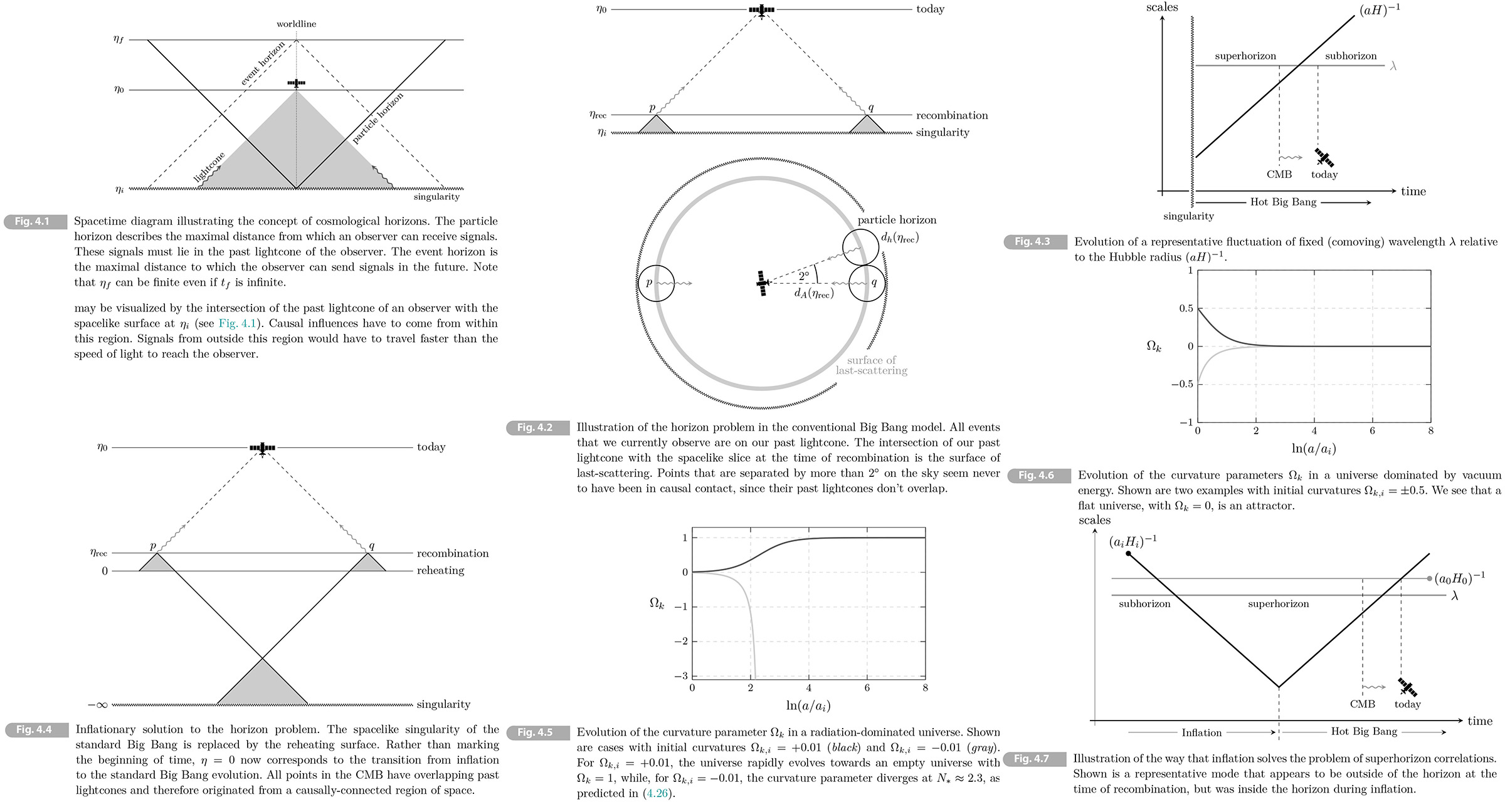
The term "particle horizon" is used to make a distinction with "event horizon" which is the maximal distance that we can influence future events, rather than the maximal distance from which we can be influenced by past events. In conventional Big Bang cosmology, we can set 𝜂𝑖 ≡ 0 and the comoving particle horizon is simply equal to the conformal time. The size of the horizon at time 𝜂 may be visualized by the intersection of past lightcone of an observer with the spacelike surface at 𝜂𝑖 (see Fig. 4.1). Causal influence have to come within this region.
Equation (4.1) can be written in the following illuminating way
(4.2) 𝑑𝘩(𝜂) = ∫𝑡𝑖𝑡 𝑑𝑡/𝑎(𝑡) = ∫𝑎𝑖𝑎 𝑑𝑎/𝑎ȧ = ∫ln 𝑎𝑖ln 𝑎 (𝑎𝐻)-1 𝑑(ln 𝑎), [= ∫ln 𝑎𝑖ln 𝑎 (𝑎𝐻)-1 𝑑(ln 𝑎)/𝑑𝑎 𝑑𝑎 = ∫𝑎𝑖𝑎 (𝑎2𝐻)-1 𝑑𝑎]
where 𝑎𝑖 ≡ 0 corresponding the BB singularity. The causal structure of the spacetime is hence related to the evolution of the comoving Hubble radius, (𝑎𝐻)-1. For ordinary matter sources, the comoving Hubble radius is a monotonically increasing function of time (or scale factor), and the integral in (4.2) is dominated by the contribution from late times. This implies that in the standard cosmology 𝑑𝘩 ~ (𝑎𝐻)-1, which has led to the confusing practice of referring to both the particle horizon and the Hubble radius as the "horizon." [Wikipedia Cosmological horizon; 𝑟HS,comoving(𝑡) = 𝑐/𝑎(𝑡)𝛨(𝑡).]
We conclude that the amount of conformal time between the initial singularity and the emission of the CMB2 was much smaller than the conformal age of the universe today, 𝜂rec ≪ 𝜂0. It means that most parts of the CMB have non-overlapping past lightcones and hence never were in causal contact. This is illustrated by the spacetime diagram in Fig. 4.2. Consider two opposite directions on the sky. The CMB photons that we receive from these directions were emitted at the point labeled 𝑝 and 𝑞 in Fig. 4.2. Wee see that the photons were released sufficiently close to the BB singularity that the past lightcones of 𝑝 and 𝑞 don't overlap. How do the photons coming from 𝑝 and 𝑞 "know" that they should be at almost exactly the same temperature? There was simply not enough time for differences in the initial temperatures to be erased by heat transfer. The same question applies to any two points in the CMB that are separated by more than 2 degrees on the sky. (anout four times the angular size of the Moon, seen from Earth). The homogeneity of the CMB spans scales that are much larger than the particle horizon when the CMB was emitted. In fact, in the standard cosmology, the CMB consists of over 40 000 causally-disconnected patches off space. Why do they looks so similar? This is the horizon problem.
To make this more explicit, consider a flat universe filled with only matter and radiation. The Friedmann equation gives us the evolution of the Hubble rate
(4.3) 𝐻2 = 𝐻02 [𝛺𝑚,0𝑎-3 + 𝛺𝑟,0𝑎-4], with 𝛺𝑟,0 = 𝑎eq𝛺𝑚,0
The comoving Hubble radius can then be written as
(4.4) (𝑎𝐻)-1 = 1/√𝛺𝑚,0 𝐻0-1 𝑎/√(𝑎 + 𝑎eq).
The conformal time as a function of scale factor then is
(4.5) 𝜂 = ∫0𝑎 𝑑(ln 𝑎)/𝑎𝐻 = 2/√𝛺𝑚,0 𝐻0-1 (√(𝑎 + 𝑎eq) - √𝑎eq). [∫0𝑎 𝑑(ln 𝑎)/𝑎𝐻 = ∫0𝑎 𝑑(ln 𝑎)/𝑑𝑎 𝑑𝑎 1/𝑎𝐻 = ∫0𝑎 1/𝑎 𝑑𝑎 1/𝑎𝐻 = ∫0𝑎 𝑑𝑎/𝑎2𝐻]
[RE Wikipedia Cosmological horizon; 𝜂 = ∫0𝑎 𝑑𝑎/𝑎2𝐻 = ∫0𝑎 1/√𝛺𝑚,0 𝐻0-1 1/√(𝑎 + 𝑎eq) 𝑑𝑎 = 2/√𝛺𝑚,0 𝐻0-1 (√(𝑎 + 𝑎eq) - √𝑎eq).]
Notice that the result has the correct limits: at early times (𝑎 ≪ 𝑎eq ≈ 3400-1), we get 𝜂 ∝ 𝑎 (as expected for the correct for the radiation-dominated era), while at late time (𝑎 ≫ 𝑎eq), we have 𝜂 ∝ 𝑎1/2 (as expected for the matter-dominated era). The conformal times today (𝑎0 = 1) and at recombination (𝑎rec ≈ 𝑎dec ≈ 1100-1) are
(4.6) 𝜂0 ≈ 2/√𝛺𝑚,0 𝐻0-1,
(4.7) 𝜂rec = 2/√𝛺𝑚,0 𝐻0-1 [√(1000-1 + 3400-1) - √3400-1] ≈ 0.00175 𝜂0.
Using the observed value of the Hubble constant, the comoving horizon at recombination is 𝑑𝘩(𝜂rec) = 𝜂rec ≈ 265 Mpc. This should be compared to the comoving distance to the surface of last-scattering, which in a flat universe is3 𝑑𝛢(𝜂rec) = 𝜂0 - 𝜂rec ≈ 𝜂0 ≈ 15.1 Gpc. The angle subtended by the horizon at recombination then is
(4.8) 𝜃𝘩 = 2𝑑𝘩(𝜂rec)/(𝜂0 - 𝜂rec) = (2 × 0.0175)/(1 - 0.0175) = 0.036 rad ≈ 2.0∘.
Including dark energy changes the distance to the surface of last-scattering by a factor of 0.9, so that 𝜃𝘩 ≈ 2.3∘.4
Although the total conformal time between the singularity and recombination is finite and small, we included times in the integral in (4.2) that were arbitrarily close to the initial singularity:
(4.9) ∆𝜂 = ∫0𝛿𝑡 𝑑𝑡/𝑎(𝑡) + ∫𝛿𝑡𝑡 𝑑𝑡/𝑎(𝑡).
However, in the first integral in (4.9) we have no reason to trust the classical geometry. We implicitly assumed that the breakdown of general relativity in the regime close to the singularity does not lead to a large contribution to the conformal time: i.e. we assumed 𝛿𝜂 ≪ ∆𝜂. This assumption may be incorrect and there may, in fact, be no horizon problem in a complete theory of quantum gravity. However, we will soon see that inflation provide a simple and computable solution to the horizon problem. Effectively, this is achieved by modifying the scale factor evolution in the second integral in (4.9), i.e. in the classical regime. We can choose this solution or a version of "quantum gravity magic".
4.1.2 The Flatness Problem
The flatness problem is closely related to the horizon problem, so that any solution to the horizon problem will also adress the flatness problem.
Let us define the time-dependent critical density of the universe as 𝜌crit(𝑡) = 3𝑀𝑃𝑙2𝐻2. [RE (2.141) and (3.2)] The time-dependent curvature parameter then is
(4.10) 𝛺𝑘 (𝑡) = (𝜌crit - 𝜌)/𝜌crit = (𝑎0𝐻0)2/(𝑎𝐻)2 𝛺 𝑘,0,
where we used that 𝜌crit ∝ 𝐻2 and (𝜌crit - 𝜌) ∝𝑎-2. [RE (2.144)] Recall that observations provide an upper bound on the size of the curvature parameter today, ∣𝛺𝑘,0∣ < 0.005. Because the comoving Hubble radius, (𝑎𝐻)-1 [= 𝑐/𝑎𝐻], is growing during the conventional hot BB, we expect that ∣𝛺𝑘∣ was even smaller in the past. Let us quantify this. Ignoring the shor period dark energy domination, the comoving Hubble radius is given by (4.4) and we can write (4.10) as
(4.11) 𝛺𝑘(𝑡) = 𝛺𝑘,0/𝛺𝑚,0 𝑎2/(𝑎 + 𝑎eq),
where we have set 𝑎0 ≡ 1. At matter-radiation equality, this implies
(4.12) ∣𝛺𝑘(𝑡eq)∣ = 𝛺𝑘,0/𝛺𝑚,0 𝑎eq/2 < 10-6.
At earlier time, the universe was dominated by radiation by radiation and we can use
(4.13) 𝐻2 = 𝐻eq2 𝛺𝑟,eq (𝑎eq/𝑎)4,
with 𝛺𝑟,eq = 0.5. The curavure parameter then becomes
(4.14) 𝛺𝑘(𝑡) = (𝑎eq𝐻eq)2/(𝑎𝐻)2 𝛺𝑘(𝑡eq) = 2𝛺𝑘(𝑡eq) (𝑎/𝑎eq)2.
Evaluating this at the time of BB nucleosynthesis, 𝑧𝛣𝛣𝑁 ≈ 4 × 10⁸, or the the electroweak phase transition, 𝑧𝐸𝑊 ≈ 1015, we find
(4.15-6) ∣𝛺𝑘(𝑡𝛣𝛣𝑁)∣ < 10-16, ∣𝛺𝑘(𝑡𝐸𝑊)∣ < 10-29.
At even earlier times, the curvature parameter is constrained to be even smaller.
A useful way of rephrasing the problem is in terms of the curvature scale 𝑅(𝑡),
(4.17) 𝑅(𝑡) = 1/√𝛺𝑘(𝑡) 𝐻-1(𝑡).
We have seen that observations constrain the curvature scale today to be 𝑅(𝑡) > 14𝐻0-1. The above constrains on 𝛺𝑘(𝑡) then imply that the curvature scale in the early universe was many orders of magnitude larger than the Hubble radius at that time. Since in the standard BB cosmology, the Hubble radius is the same order as the particle horizon, this suggest a fine-tuning of many causally-disconnected patches of space. Section 2.3.5 [Friedmann Equation] relates the spatial curvature of a region of space to sum of kinetic and potential energies in the region. The flatness problem can therefore also be viewed as the problem of adjusting the initial velocities of all particles over distances that naively have never been in causal contact.
4.1.3 Superhorizon correlations
A new theory of he initial condition of the universe might dismiss the horizon and flatness problem. What cannot be dismissed, however, is the fact that the universe contains density fluctuations that are correlated over apparently acausal distances. This modern version of horizon problem begs for a dynamical explanation.
To understand the severity of the problem, let us consider the fluctuations that w e observe in th CMB and in large-scale structure of the universe. Fig. 4.1 shows the evolution of a representative fluctuation of wavelength 𝜆 relative to the Hubble radius (𝑎𝐻)-1. In comoving coordinates, wavelength 𝜆 is fixed and the Hubble radius increase. This means that any fluctuation that is inside the Hubble radius today was outside the Hubble radius at sufficiently early times. For the standard hot BB, the Hubble radius is approximately equal to the particle horizon, so we call these regimes "subhorizon" and "superhorizon". Avobe we saw that the particle horizon at recombination was about 265 Mpc. Scales larger than this would not have been inside the horizon before the CMB was emitted. Yet, we find the CMB fluctuations to be correlated on scales that are larger than this apparent horizon. Not only is the CMB homogeneous on apparently acausal scale, this modern version of horizon problem also has correlated fluctuations on these scale.
4.2 Before the Hot Bing Bang
The causality issues described above suggested that there was a phase before the hot Big Bang during which the homogeneity of the univesr and its correlated fluctuations were generated.
4.2.1 A Shrinking Hubble Sphere
Our description of the horizon and flatness problems gas highlighted the fundamental role played by the growing comoving Hubble radius of the standard BB cosmology. A simple solution to these problem therefore suggests itself: let us conjecture a phase of decreasing comoving Hubble radius in the early universe.
(4.18) 𝑑/𝑑𝑡 (𝑎𝐻)-1 < 0.
The shrinking Hubble sphere as the fundamental definition of inflation is preferred since it relates most directly to the horizon problem and is also a key feature of the inflationary mechanism for generating fluctuations (see Chapter 8). Using 𝑎𝐻 = ȧ, it is easy to see that this is equivalent to ä > 0, leading to the familiar notion of inflation as a period of accelerated expansion. If inflation lasts long enough, then the horizon and flatness problems can be avoided.
It will now be important to distinguish clearly between particle horizon and the Hubble radius. The
Hubble radius is the distance that particles can travel in the course of one expansion time, 𝐻-1, which is roughly the time in which the scale factor doubles. The Hubble radius is another way of measuring whether particles are causally connected with each other: Particles that are separated by distances greater than the particle horizon could never have communicated with one another. Inflation is a mechanism to make the particle horizon much larger than the Hubble radius. This means that the particles can't communicate now, but were in causal contact early on,
4.2.2 Horizon Problem Revisited
Consider again the expression (4.2) for comoving particle horizon
(4.19) 𝑑𝘩(𝜂) = ∫ln 𝑎𝑖ln 𝑎 (𝑎𝐻)-1 𝑑(ln 𝑎).
In the standard BB cosmology, the integral is dominated by late times and the particle horizons is the same order as the Hubble radius, 𝑑𝘩(𝜂) ~ (𝑎𝐻)-1. However, if the comoving Hubble radius is instead a decreasing function of time, then the integral is dominated by early times and the particle horizon can be much larger than the Hubble radius, 𝑑𝘩(𝜂) ~ (𝑎𝑖𝐻𝑖)-1 ≫ (𝑎𝐻)-1. As we will see, that is precisely what the doctor ordered.
To illustrate this further, consider a flat universe dominated by a fluid with a consit equation of state 𝜔 ≡ 𝑃/𝜌. [= 𝑃/(𝜌𝑐2) (2.107)] From
the Friedmann equation, we infer that the evolution of the comoving Hubble radius is [RE (2.148)]
(4.20) (𝑎𝐻)-1 = 𝐻0-1 𝑎1/2 (1 + 3𝜔),
and the comoving particle horizon becomes
(4.21) 𝑑𝘩(𝑎) = 2𝐻0-1/(1 + 3𝜔) [𝑎1/2 (1 + 3𝜔) - 𝑎𝑖1/2 (1 + 3𝜔)] ≡ 𝜂 - 𝜂𝑖.
Ordinary matter satisfies the strong energy condition (SEC), 1 + 3𝜔 > 0, so that the Hubble radius grows and the particle horizon is dominated by late time, 𝑎 ≫ 𝑎𝑖 and get 𝑑𝘩 = 𝜂. Now, take 1 + 3𝜔 < 0 instead. The Hubble radius then shrunk and the particle horizon receives most of its contribution from early times. In fact, we now have
(4.22) 𝜂𝑖 ≡ 2𝐻0-1/(1 + 3𝜔) 𝑎𝑖1/2 (1 + 3𝜔) → [𝑎𝑖 → 0, 𝜔 <-1/3] → -∞.
The BB singularity has been pushed to negative conformal time, so that there was actually much more conformal time between the singularity and recombination than we had thought.
Fig. 4.4 shows that the new spacetime diagram. Let us denote the beginning and the end of inflation by 𝜂𝑖 and 𝜂𝑒, respectively. If ∣𝜂𝑒 - 𝜂𝑖∣ ≫ 𝜂0 - 𝜂rec, then the past lightcones of widely separated points in the CMB had enough time to intersect. The uniformity of the CMB is not a mystery anymore. In inflationary cosmology, 𝜂 = 0 is not the initial singularity, but instead is only a transition point between inflation and the hot BB. There is time before and after 𝜂 = 0.5
4.2.3 Flatness Problem Revisited
Next, we show how the shrinking Hubble sphere also solves the flatness problem. We have seen that the evolution of the curvature parameter is related to the evolution of the comoving Hubble radius as
(4.23) 𝛺𝑘(𝑡) = (𝑎𝑖𝐻𝑖)2/(𝑎𝐻)2 𝛺𝑘(𝑡𝑖).
Any initial curvature will therefore decrease, if the comoving Hubble radius decreases. If the inflation lasts long enough it therefore solves the flatness problem.
Let us consider the case of a perfect fluid with a constant equation of state 𝜔. The Friedmann equation then implies
(4.24) (𝑎𝐻)2 = (𝑎𝑖𝐻𝑖)2 [(1 - 𝛺𝑘,𝑖)(𝑎/𝑎𝑖)-(1 + 3𝜔) + 𝛺𝑘,𝑖],
and substituting this into (4.23), we get
(4.25) 𝛺𝑘(𝑁) = 𝛺𝑘,𝑖𝑒(1 + 3𝜔)𝑁/[(1 - 𝛺𝑘,𝑖) + 𝛺𝑘,𝑖𝑒(1 + 3𝜔)𝑁],
where 𝑁 ≡ ln(𝑎/𝑎𝑖) is the number of "e-folds" of expansion. This solution has two fixed points at 𝛺𝑘,𝑖 = 0 (a flat universe) and 𝛺𝑘,𝑖 = 1 (an empty Milne universe). Fig 4.5 shows the evolution of 𝛺𝑘 for a radiation-dominated universe. [RE (2.144) 𝛺𝑘 > 0 for 𝑘 < 0] With 1 + 3𝜔 > 0, any deviation from 𝛺𝑘 = 0 is unstable and grows with time. For a negative curved universe (with 𝛺𝑘 > 0), the growth then slows as 𝛺𝑘 approaches its second fixed point at 𝛺𝑘 = 1. This final state is an empty universe with negative curvature. For a positively curved universe (with 𝛺𝑘 < 0), the growth accelerates and the curvature parameter diverges at
(4.26) 𝑁* = 1/(1 + 3𝜔) ln ∣𝛺𝑘,𝑖 -1/𝛺𝑘,𝑖∣.
The divergence occurs when the Hubble parameter vanishes, cf. (4.24), and therefore corresponds to the turn-around point of the scale factor (see Fig. 2.12).
Exercise 4.1 Show that the curvature parameter in (4.23) satisfies the following evolution equation
(4.27) 𝑑𝛺𝑘/𝑑𝑁 = (1 + 3𝜔) 𝛺𝑘 (1 - 𝛺𝑘).
This makes it transparent that 𝛺𝑘 = 0 and 𝛺𝑘 =1 are fixed points, and that the behavior away from these points depends on the equation of state.
[Solution] (4.23) 𝛺𝑘(𝑡) = (𝑎𝑖𝐻𝑖)2/(𝑎𝐻)2 𝛺𝑘(𝑡𝑖); Setting 𝑁 = ln (𝑎𝑖𝐻𝑖)2𝑎 and 𝜔 = 𝑃/𝜌𝑐2
(a) 𝑑𝛺𝑘/𝑑𝑁 = 𝑑𝑡/𝑑[ln (𝑎𝑖𝐻𝑖)2𝑎] 𝑑𝛺𝑘/𝑑𝑡 = 1/[ln (𝑎𝑖𝐻𝑖)2𝐻] 𝛺𝑘 𝑑(ln 𝑑𝛺𝑘)/𝑑𝑡 = -2 𝛺𝑘/𝐻 𝑑(ln ȧ)/𝑑𝑡 = -2 𝛺𝑘/𝐻 ä/ȧ = -2𝛺𝑘 ä/𝑎𝐻2.
Using Friedmann equations,
(b) 𝐻2 = 8π𝐺/3 𝜌 - 𝑘𝑐2/𝑎2𝑅02 = 8π𝐺/3 𝜌 + 𝐻2𝛺𝑘.
(c) ä/𝑎 = -4π𝐺/3 (𝜌 + 3𝑃/𝑐2) = -4π𝐺/3 𝜌(1 + 3𝜔) = 𝐻2/2 (1 - 𝛺𝑘)(1 + 3𝜔).
Substituting (c) to (a), we get
(d) 𝑑𝛺𝑘/𝑑𝑁 = (1 + 3𝜔) 𝛺𝑘 (1 - 𝛺𝑘). ▮
The evolution of the curvature parameter is drastically different if the fluid violates the strong energy condition (SEC), 1 + 3𝜔 < 0. The solution in (4.25) still applies and shows that ∣𝛺𝑘∣ decreases as 𝑒-∣1 + 3𝜔∣𝑁, so that the fixed point 𝛺𝑘 = 0 is now an attractor (see Fig. 4.6). The flatness problem is solved if the inflationary expansion lasts long enough to reduce any initial curvature to such a low value at the beginning of the hot BB that the subsequent expansion doesn't increase it above the observational bound of ∣𝛺𝑘,0∣ < 0.005. In practice, that this means between 40 and 60 𝑒-folds of inflationary expansion (see Section 4.2.5).
4.2.4 Superhorizon Correlations
The shrinking Hubble sphere also explain how the fluctuations observed in the CMB can be correlated on apparently superhorizon scales. Fig. 4.7 shows the evolution of a fixed comoving scale relative to the Hubble radius. If inflaion lasted long enough, this scale started its life inside the Hubble radius, wherecausal processes were able to create nontrivial correlations. The fluctuations then exited the Hubble radius6 and are measured today as apparently superhorizon correlations in the CMB. Notice the symmetry of the evolution. Scales just entering the Hubble radius today, 60 𝑒-folds after the end of inflation, left the Hubble radius 60 𝑒-folds before the end of inflation.
4.2.5 Duration of Inflation
How much inflation is needed o solve the problems of the hot BB? Since the Hubble radius is easier to calculate than the particle horizon, it is common to use the Hubble radius as a means of judging the causality problem. The problems are solved if the entire observable universe is smaller than the comoving Hubble radius at the beginning of inflation (see Fig. 4.7).
(4.28) (𝑎0𝐻0)-1 < (𝑎𝑖𝐻𝑖)-1
Notice that this is more conservative than using the particle horizon, since 𝑑𝘩(𝑡𝑖) is bigger than (𝑎𝑖𝐻𝑖)-1. We don't have to assume anything about earlier times 𝑡 < 𝑡𝑖, while 𝑑𝘩(𝑡𝑖) depends on the entire history of time before inflation.
The physical Hubble rate is nearly constant during inflation, so that 𝐻𝑖 ≈ 𝐻𝑒. During infaltion the scale factor increase while the comoving Hubble radius is decrease. The latter is typically expressed in terms of the number of 𝑒-foldings
(4.29) 𝑁tot ≡ ln(𝑎𝑒/𝑎𝑖).
We would like to detertime the minimal number of 𝑒-foldings that is required to solve the problem of hot BB.
As in Fig. 4.7, the decrease of the comoving Hubble radius during inflation must compensate for its increase during the hot BB. The amount grown during the hot BB depends on the maximal temperature of the thermal plasma at the beginning of the hot BB. We will denote this so-called reheating temperature by 𝛵𝑅. We take the universe to be radiation-dominated throughout. Remembering that 𝐻 ∝ 𝑎-2 during the radiation-dominated era, we have
(4.30) 𝑎0𝐻0/𝑎𝑅𝐻𝑅 = 𝑎0/𝑎𝑅 (𝑎𝑅/𝑎0)2 = 𝑎𝑅/𝑎0 ~ 𝛵0/𝛵𝑅 ~ 10-28 (1015 GeV/𝛵𝑅),
where we have introduce a reference, 1015 GeV for the reheating temperature. We will furthermore assume that the energy density at the end of inflation was converted relatively quickly into the particles of thermal plasma, so that the Hubble radius didn't significantly grow between the end of inflation and the beginning of hot BB, (𝑎𝑒𝐻𝑒)-1 ~ (𝑎𝑅𝐻𝑅)-1. The condition can then written as
(4.31) (𝑎𝑖𝐻𝑖)-1 > (𝑎0𝐻0)-1 ~ 10-28 (𝛵𝑅/1015 GeV) 𝑎𝑒𝐻𝑒)-1,
and using 𝐻𝑖 ≈ 𝐻𝑒, we get
(4.32) 𝑁tot ≡ ln(𝑎𝑒/𝑎𝑖) > 64 + ln(𝛵𝑅/1015 GeV).
This is the famous statement that the solution of the horizon problem requires about 60 𝑒-folds of inflation. Notice the fewer 𝑒-folds are needed if the reheating temperature is lower.
1 Notice that the Big Bang singularity is a moment in time, not a point in space. In Fig. 4.1-2 we depict the singularity by an extended (possibly infinite) spacelike hypersurface.
2 In this chapter we don't distinguish between recombination and photon decoupling and simply refer to boths as 'recommbination."
3 Notice that we used the same notation, 𝑑𝛢, for the physical angular diameter distance in Section 2.2.3.
4 As we will see in Chapters 6 and 7, fluctuations in primordial plasma actually propagate at the speed of sound, which is smaller than the speed of light, 𝑐𝑠 = 𝑐/√3. The angular size of the corresponding sound horizon is 𝜃𝑠 = 𝜃𝘩/√3 ≈ 1.3∘, which explains why the pattern of CMB fluctuations has special features n the scale of 1 degree.
5 Notice that the BB singularity is still at 𝑡 = 0. The time between the singularity and recombination is fixed, but the lightcones get stretched drastically by the inflationary expansion.
6 We will later refer the Hubble radius as "horizon", but it is important to keep in mind that the Hubble radius and the horizon are vastly different during inflation.
|
|
|