|
김관석
|
2024-10-06 19:11:13, 조회수 : 109 |
- Download #1 : BC_5a.jpg (119.2 KB), Download : 0

Part II The Inhomogeneous Universe
5 Structure Formation
To understand the large-scale structure of the universe, we have to introduce inhomogeneities and follow their evolution. As long as the perturbations remain relatively small, we can treat them in perturbation theory. We will develop the formalism of cosmological perturbation theory, first in Newtonian gravity in this chapter and then in full GR in the next chapter.
For most of the history of the universe, the growth of structure was dominated by the evolution of dark mater. Although the microscopic nature of the dark matter is still unknown, its long-wavelength properties are captured by a small number of parameters, such as an equation of state and a sound speed. The insensitivity of the physics at long distances to effects on small scales is a general feature of most physical systems. Physics has progressed because we can study "effective theories" that are valid for a certain range of scales and coarse grain over the microscopic details. This means that the fluctuations in the unknown dark matter obey the equation of fluid mechanics. We would like to understand what happens when this fluid is perturbed.
5.1 Newtonian Perturbation Theory
Newtonian gravity is a good approximation with small velocities compared to the speed of light and the departures from a flat spacetime geometry are small. The latter is satisfied on scales smaller than the Hubble radius, 𝐻-1. The treatment of this section will be restricted to sub-Hubble fluctuations in non-relativistic matter.
5.1.1 Fluid Dynamics
Consider a fluid with a mass density 𝜌, pressure 𝑃 ≪ 𝑃 and velocity 𝐮. We will first study the evolution of perturbations in this fluid while ignoring gravity and the expansion of the universe. In the following sections, we will add these complications.
Mass conservation implies the continuity equation
(5.1) ∂𝜌/∂𝑡 + 𝛁 ⋅ (𝜌𝐮) = 0.
This equation simply reflects the fact that the mass density in a fixed volume can only change if there is a flux of a particles leaving or entering the volume. Momentum conservation leads to the Euler equation (see Problem 5.1): [RE Wikipedia Euler equations (fluid dynamics)]
(5.2) 𝜌 𝑑𝐮/𝑑𝑡 = 𝜌(∂/∂𝑡 + 𝐮 ⋅ 𝛁)𝐮 = -∇𝑃,
which is simply "𝐹 = 𝑚𝑎" for fluid element. Notice that the acceleration is not given by ∂𝑡𝐮, but the "convective time derivative" (∂𝑡 + 𝐮 ⋅ ∇)𝐮 in which follows the fluid element as it moves. To close the system of equations, we also have to specify an equation of state:
(5.3) 𝑃 = 𝑃(𝜌, 𝛵),
For a static of fluid, with 𝐮 = 0, the above equations simply imply a constant density and pressure, 𝜌 = 𝜌̄ and 𝑃 = 𝑃̄. We take ∣𝐮∣ ≪ 𝑐, and write
(5.4-5) 𝜌(𝑡, 𝐱) = 𝜌̄ + 𝛿𝜌(𝑡, 𝐱), 𝑃(𝑡, 𝐱) = 𝑃̄ + 𝛿𝑃(𝑡, 𝐱).
As long as all perturbation are small, we can "linearize" the fluid equations. Linearizing means: Consider a product of two quantities 𝛢 and 𝛣. Expanding each factor into a background value and perturbation, we get
(5.6) 𝛢𝛣 = (𝛢̄ + 𝛿𝛢)(𝛣̄ + 𝛿𝛣) = 𝛢̄𝛣̄ + 𝛢̄𝛿𝛣 + 𝛿𝛢𝛣̄ + 𝛿𝛢𝛿𝛣.
The result has three sets of terms: 𝛢̄𝛣̄ contains only background quantities and is therefore called zeroth order in perturbations; 𝛢̄𝛿𝛣 + 𝛿𝛢𝛣̄ is first order in perturbations; 𝛿𝛢𝛿𝛣 is a product of two perturbations and hence is called second order. Linearizing the equation means dropping all terms that are higher than first order in perturbations. This means writing
(5.7) 𝛢𝛣 ≈ 𝛢̄𝛣̄ + 𝛢̄𝛿𝛣 + 𝛿𝛢𝛣̄.
The linearized answer is a good approximation to the true answer.
Applying this procedure to the continuity equation (5.1) and the Euler equation (5.2), we get
(5.8-9) ∂𝑡𝛿𝜌 = -𝛁 ⋅ (𝜌̄𝐮), 𝜌̄𝐮∂𝑡𝐮 = -𝛁𝛿𝑃.
Combining ∂𝑡 (5.8) and 𝛁 ⋅ (5.9) gives
(5.10) ∂𝑡2𝛿𝜌 - ∇2𝛿𝑃 = 0.
For simplicity, we will consider a barotropic fluid, such that 𝑃 = 𝑃(𝜌). In that case, we can write the pressure perturbation as
(5.11) 𝛿𝑃 = ∂𝑃/∂𝜌 𝛿𝜌 ≡ 𝑐𝑠2𝛿𝜌,
where 𝑐𝑠 is the sound speed of the fluid, Equation (5.10) then takes the form
(5.12) (∂2/∂𝑡2 - 𝑐𝑠2∇2)𝛿𝜌 = 0.
This is a wave equation and it solution are sound waves
(5.13) 𝛿𝜌(𝐱, 𝑡) = 𝛢𝐤 sin(𝜔𝑡 - 𝐤 ⋅ 𝐱) + 𝛣𝐤 cos(𝜔𝑡 - 𝐤 ⋅ 𝐱).
where 𝐤 is the wavevector and 𝜔 = 𝑐𝑠∣𝐤∣ is the frequency. The wavevector points in the wave's direction of travel and its magnitude is inversely related to wavelength 𝜆 = 2π/∣𝐤∣. Since (5.12) is a linear equation, we can add solutions with different wavevectors 𝐤.
The more formal way of solving a partial differential equation (PDE) like (5.12) is to write 𝛿𝜌 as a Fourier expression
(5.14) 𝛿𝜌(𝐱, 𝑡) = ∫ 𝑑3𝑘/(2π)2 𝑒𝑖𝐤 ⋅ 𝐱 𝛿𝜌(𝐤, 𝑡).
Acting with a spatial derivative ∂𝑖 pulls down a factor of 𝑖𝐤 from 𝑒𝑖𝐤 ⋅ 𝐱 and the Laplacian in (5.12) become -𝑘2, with 𝑘 ≡ ∣𝐤∣, in Fourier space. This turns the wave equation into an ordinary equation (ODE) for each Fourier mode
(5.15) (∂2/∂𝑡2 + 𝑐𝑠2𝑘2)𝛿𝜌(𝐤, 𝑡) = 0.
The solution for each Fourier mode then is
(5.16) 𝛿𝜌(𝐤, 𝑡) = 𝐶𝐤 𝑒-𝑖𝜔𝑘 𝑡 + 𝐷𝐤 𝑒𝑖𝜔𝑘 𝑡,
with 𝜔𝑘 ≡ 𝑐𝑠𝑘. Substituting this back into (5.14) gives
(5.17) 𝛿𝜌(𝐱, 𝑡) = ∫ 𝑑3𝑘/(2π)2 [𝐶𝐤 𝑒-𝑖(𝜔𝑘 𝑡 - 𝐤 ⋅ 𝐱) + 𝐷𝐤 𝑒𝑖(𝜔𝑘 𝑡 + 𝐤 ⋅ 𝐱)]
= ∫ 𝑑3𝑘/(2π)2 [𝐶𝐤 𝑒-𝑖(𝜔𝑘 𝑡 - 𝐤 ⋅ 𝐱) + 𝐷-𝐤 𝑒𝑖(𝜔𝑘 𝑡 - 𝐤 ⋅ 𝐱)]
= ∫ 𝑑3𝑘/(2π)2 [𝐶𝐤 𝑒-𝑖(𝜔𝑘 𝑡 - 𝐤 ⋅ 𝐱) + 𝐶*𝐤 𝑒𝑖(𝜔𝑘 𝑡 - 𝐤 ⋅ 𝐱)].
The latter is required in order for 𝛿𝜌(𝐱, 𝑡) to be real. Defining 𝐶𝐤 ≡ [𝛣𝐤 + 𝑖𝛢𝐤]/2 we can also write this as
(5.18) 𝛿𝜌(𝐱, 𝑡) = ∫ 𝑑3𝑘/(2π)2 [𝛢𝐤 sin(𝜔𝑘 𝑡 - 𝐤 ⋅ 𝐱) + 𝛣𝐤 cos(𝜔𝑘 𝑡 - 𝐤 ⋅ 𝐱),
which shows that the most general solution to the wave equation is indeed a sum over the plane wave solutions in (5.13).
5.1.2 Adding Gravity
Let us now turn on gravity, but still keep the spacetime static. Later we will fix the spacetime to be dynamical.
The continuity equation (5.1) remains unchanged, but the Euler equation (5.2) receives an extra force term
(5.19) 𝜌(∂/∂𝑡 + 𝐮 ⋅ 𝛁)𝐮 = -𝛁𝑃 - 𝜌𝛁𝛷,
where 𝛷 is the gravitational potential. The potential is determined by the local density the Poisson equation
(5.20) ∇2𝛷 = 4π𝐺𝜌.
For a static fluid with 𝐮 = 0, equations (5.1) and (5.19) are again solved by a constant density and pressure, 𝜌 = 𝜌̄ and 𝑃 = 𝑃̄. However, this implies that ∇𝛷̄ = 0, which is not consistent with the Poisson equation (5.20). This is a reflection of the fact that there are no infinite, static, self-gravitating fluids.
Although we have't found a consistent solution for the background, the linearized continuity and Euler equations now are
(5.21-2) ∂𝑡𝛿𝜌 = -𝛁 ⋅ (𝜌̄𝐮), 𝜌̄𝐮∂𝑡𝐮 = -𝛁𝛿𝑃 - 𝜌̄𝛁𝛿𝛷,
where 𝛿𝛷 = 𝛷 - 𝛷̄, which satisfies
(5.23) ∇2𝛿𝛷 = 4π𝐺𝛿𝜌
As before, these equations can be combined into a single equation for density fluctuation:
(5.24) (∂2/∂𝑡2 - 𝑐𝑠2∇2 - 4π𝐺𝜌̄)𝛿𝜌 = 0.
so that each Fourier ode now obeys
(5.25) (∂2/∂𝑡2 - 𝑐𝑠2𝑘2 - 4π𝐺𝜌̄)𝛿𝜌(𝐤, 𝑡) = 0.
We see that there is a critical wavenumber, called the Jean scale, for which the frequancy of oscillation is zero:
(5.26) 𝑘𝐽 ≡ √(4π𝐺𝜌)/𝑐𝑠.
The nature of the solution depends on the size of the wavenumber 𝑘 relative to 𝑘𝐽. For large wavenumber, 𝑘 ≫ 𝑘𝐽, the pressure dominates and we find the same oscillations as before. However, on large scale, 𝑘 < 𝑘𝐽, gravity dominates and (5.25) becomes
(5.27) (∂2/∂𝑡2 - 4π𝐺𝜌̄)𝛿𝜌 = 0.
The solutions to this equation take the form 𝛿𝜌 ∝ exp(±𝑡/𝜏), where 𝜏 ≡ 1/√(4π𝐺𝜌). The exponential growth of the fluctuation is called the Jeans instability.
5.1.3 Adding Expansion
Finally, we will account the expansion of the universe. We do this by interpreting the coordinates appearing in the fluid equations as physical coordinates 𝐫, and write them in terms of the comoving coordinates 𝐱,
(5.28) 𝐫(𝑡) = 𝑎(𝑡)𝐱.
The velocity field is given by
(5.29) 𝐮(𝑡) = ṙ = 𝐻𝐫 + 𝐯.
where 𝐻𝐫 is the Hubble flow and 𝐯 = 𝑎ẋ is the (physical) peculiar velocity. In a static spacetime, the derivative ∂𝑡 and 𝛁 are independent, while in an expanding spacetime they are not. Consider, for example, derivative of a function 𝑓(𝑡, 𝐫) = 𝑓(𝑡, 𝑎(𝑡)𝐱) at fixed 𝐱,
(5.30) (∂𝑓/∂𝑡)𝐱 = (∂𝑓(𝑡, 𝑎(𝑡)𝐱)/∂𝑡)𝐱 = (∂𝑓/∂𝑡)𝐫 + ∂𝑎(𝑡)𝐱)/∂𝑡 ⋅ (∂𝑓/∂𝐫) = [(∂𝑓/∂𝑡)𝐫𝑡 + 𝐻𝐫 ⋅ 𝛁𝐫]𝑓,
where 𝛁𝐫 is the gradient with respect to 𝐫 at fixed 𝑡. In terms of 𝛁𝐱, the gradient with respect to 𝐱, we have 𝛁𝐫 = 𝑎-1𝛁𝐱. Equation (5.30) can also be written as
(5.31) (∂𝑓/∂𝑡)𝐫 = [(∂𝑓/∂𝑡)𝐱 - 𝐻𝐱 ⋅ 𝛁𝐱]𝑓. [verification needed]
With this in mind, let us look at the fluid equations in an expanding universe.
• Applying these substitutions to the continuity equation (5.1), we get
(5.32) (∂𝜌/∂𝑡)𝐫 + 𝛁𝐫 ⋅ (𝜌𝐮) = 0, [(∂𝑓/∂𝑡)𝐱 - 𝐻𝐱 ⋅ 𝛁𝐱]𝜌 + 1/𝑎 ∇𝐱 ⋅ (𝜌𝐮) = 0.
Using (5.29) for 𝐮 then gives
(5.33) ∂𝜌/∂𝑡 + 3𝐻𝜌 + 1/𝑎 𝛁 ⋅ (𝜌𝐯) = 0, [verification needed]
[(∂/∂𝑡) - 𝐻𝐱 ⋅ 𝛁]𝜌 + 1/𝑎 𝛁 ⋅ (𝜌𝐮) = [(∂/∂𝑡) - 𝐻𝐱 ⋅ 𝛁]𝜌 + 1/𝑎 𝛁 ⋅ [𝜌(𝐻𝐫 + 𝐯)] = ∂𝜌/∂𝑡 - 3𝐻𝜌 + 1/𝑎 𝛁 ⋅ [𝜌(𝐻𝑎𝐱 + 𝐯)] = ∂𝜌/∂𝑡 - 3𝐻𝜌 + 3𝐻𝜌 + 1/𝑎 𝛁 ⋅ (𝜌𝐯) = ∂𝜌/∂𝑡 + 1/𝑎 𝛁 ⋅ (𝜌𝐯) = 0.]
where we omit the subscripts 𝐱 and used 𝛁 ⋅ 𝐱 =3. In the following, all the time derivatives will be at fixed 𝐱 and ∇ will always stands for ∇𝐱.
• Similar manipulation of the Euler equation (5.19) lead to
(5.34) (∂/∂𝑡 + 𝐯 ⋅ 𝛁)𝐮 = -1/𝑎 𝛁𝑃/𝜌 - 1/𝑎 𝛁𝛷
where we have use (5.31) and (5.29).
• The Poisson equation (5.20) simply becomes
(5.35) ∇2𝛷 = 4π𝐺𝑎2𝜌,
where 𝑎2 accounts for the difference between physical and comoving distances.
Our task is to solve the coupled equations (5.33), (5.34) and (5.35). We again first find the background solution and then consider linear perturbations.
• Background solution: Setting 𝐯 = 0, we get
(5.36) ∂𝜌̄/∂𝑡 = -3𝐻𝜌.
(5.37) ∂𝐮̄/∂𝑡 = -1/𝑎 ∇𝑃̄/𝜌̄ - 1/𝑎 ∇𝛷̄.
Equation (5.36) is the familiar continuity equation for a homogeneous non-relativistic fluid. Therefore background density 𝜌̄ ∝ 1/𝑎3, as expected. The Euler equation (5.37) has the following solution
(5.38) 𝐮̄ = 𝐻𝑎𝐱, 𝑃̄ = const, ∇𝛷̄ = -ä𝑎𝐱.
This solution is now consistent with the Poisson equation,
(5.39) ä/𝑎 = -4π𝐺/3 𝜌̄,
which is the second Friedmann equation.
• Linear perturbations: Next, we introduce perturbation around the background solution
(5.40) 𝜌 = 𝜌̄[1 + 𝛿], 𝐮 = 𝐻𝑎𝐱 + 𝐯, 𝑃 = 𝑃̄ + 𝛿𝑃, 𝛷 = 𝛷̄ + 𝛿𝛷,
where the density contrast is
(5.41) 𝛿 ≡ 𝛿𝜌/𝜌̄.
As long as 𝛿 ≪ 1, we can linearize the equations.
Expanding the continuity equation (5.33) to linear order in the fluctuation, we find
(5.42) ∂(𝜌̄𝛿)/∂𝑡 + 3𝐻𝜌̄𝛿 + 1/𝑎 𝛁 ⋅ (𝜌̄𝐯) = 0.
Using (5.36) we obtain the following for the density contrast
(5.43) 𝛿̇ = -1/𝑎 𝛁 ⋅ 𝐯.
We see that the growth of the density perturbations is sourced by the divergence of the fluid velocity. At linear order, the vorticity of the fluid, 𝛁 × 𝜔, therefore doesn't contribute.
Similarly linearizing the Euler equation (5.34) gives
(5.44) 𝐯̇+ 𝐻𝐯 = -1/𝑎𝜌̄ 𝛁𝑃𝛿 - 1/𝑎 ∇𝛿𝛷,
where we have used that (𝐯 ⋅ 𝛁)𝐱 = 𝐯.[verification needed] In the absence of pressure and gravitational perturbations, this equation simply says that 𝐯 ∝ 𝑎-1.[verification. needed]
As before, it will be instructive to combine two first-order equations (5.43) and (5.34) into a single second-order equation. First, we take the time derivative of (5.43) to get
(5.45) 𝑑𝛿̇/𝑑𝑡 - 𝐻/𝑎 𝛁⋅ 𝐯 + 1/𝑎 𝛁⋅ 𝐯̇ = 0.
Substituting (5.44) for ύ and (5.43) for 𝛁⋅ 𝐯, this becomes
(5.46) 𝑑𝛿̇/𝑑𝑡 + 2𝐻𝛿̇ - 1/𝑎2 (1/𝜌̄ ∇2𝛿𝑃 + ∇2𝛿𝛷 = 0.
Finally, we use 𝛿𝑃 = 𝑐𝑠2𝜌̄𝛿 for the pressure perturbation and ∇2𝛿𝛷 = 4π𝐺𝑎2𝜌̄𝛿 for the gravitational potential. The final form of our evolution equation for the density contrast is
(5.47) 𝑑𝛿̇/𝑑𝑡 + 2𝐻𝛿̇ - [𝑐𝑠2/𝑎2∇2 + 4π𝐺𝜌̄(𝑡)]𝛿 = 0.
This is the main equation describing the growth of density fluctuations in an expanding universe.
5.2 Growth of Matter Perturbation
Two important example for non-relativistic fluids are cold dark-matter and baryons after decoupling. In this section,we will study the evolution of fluctuations in these fluids.
5.2.1 Jeans Instability
Now we will show how the nature of Jeans instability is modified by the expansion of the universe.It is convenient to study the evolution in Fourier space, so that (5.47) becomes
(5.48) 𝑑𝛿̇/𝑑𝑡 + 2𝐻𝛿̇ - 𝑐𝑠2 (𝑘2/𝑎2 - 𝑘𝐽2) 𝛿(𝐤, 𝑡) = 0,
where we introduces the physical Jeans wavenumber
(5.49) 𝑘𝐽(𝑡) ≡ √(4π𝐺𝜌̄(𝑡)/𝑐𝑠(𝑡).
We see that the Jeans scale takes the same form as in (5.26), but now depends on time through the evolution of 𝜌̄(𝑡) and possibly 𝑐𝑠(𝑡).
On small scales, 𝑘/𝑎 ≫ 𝑘𝐽, equation (5.48) reduces to the equation of a damped harmonic oscillator with a friction term, 2𝐻𝛿̇, provided by the expansion of the universe. On large scales, 𝑘/𝑎 ≪ 𝑘𝐽, we can ignore the pressure term and (5.48) becomes [Wikipedia Harmonic oscillator]
(5.50) 𝑑𝛿̇/𝑑𝑡 + 2𝐻𝛿̇ - 4π𝐺𝜌̄(𝑡)𝛿 = 0. [with 𝛿̇ ≡ 𝑑𝛿/𝑑𝑡]
which should be compared to (5.27) in static space. A consequence of the extra friction term is that the fluctuation now don't grow exponentially.
For baryon, the sound speed and hence the Jeans scale are strong function of time, Before recombination, the baryons are strongly coupled to the photons, forming a relativistic photon-baryon fluid with 𝑐𝑠(𝑡) ≈ 1/√3. The Jeans scale is then the order of the Hubble radius, so that there is no growth of baryonic fluctuations o subhorizon scales. After recombination, the sound speed of the baryon fluid drops drastically and its fluctuations start to grow.
For cold dark matter, the sound speed is negligible at all times, so that subhorizon modes can start to grow earlier. The detail of the growth depend on the evolution of the background density.
5.2.2 Linear Growth Function
The density contrast satisfies the second order linear ODE (5.50) involving only time derivatives. Any solution of (5.50) can be written as
(5.51) 𝛿(𝐤, 𝑡) = 𝛿+(𝐤)𝐷+(𝑡) + 𝛿-(𝐤)𝐷-(𝑡).
where 𝛿±(𝐤) are the Fourier modes of the initial density field and the 𝑘-independent function 𝐷±(𝑡) describes the linear evolution. We refer to 𝐷+(𝑡) and 𝐷-(𝑡) as the growing and decaying modes, respectively. The growing mode is often called the linear growth function and is normalized so that 𝐷+(𝑡0) ≡ 1. The functional form of 𝐷±(𝑡) will depend on the evolution of the background density.
Let us to start with the case of matte perturbations in a flat matter-dominated universe. After matter-radiation equality since 𝑎 ~ 𝑡2/3, we have
(5.52) 𝐻(𝑡) = 2/3𝑡, 4π𝐺𝜌̄𝑚(𝑡) = 3/2 𝐻2 = 2/3𝑡2 [RE Friedmann equations]
hence (5.50) leads to
(5.53) 𝑑Ḋ/𝑑𝑡 + 4/3𝑡 Ḋ - 2/3𝑡2 𝐷 = 0.
The two solutions of this equation are
(5.54) 𝐷-(𝑡) ∝ 𝑡-1 ∝ 𝑎-3/2, 𝐷+(𝑡) ∝ 𝑡2/3 ∝ 𝑎,
so that the density contrast grows in proportion to the scale factor, 𝛿 ∝ 𝑎. Note that this means that the density fluctuation 𝛿𝜌 is still decreasing, since 𝛿𝜌 = 𝜌̄𝛿 ∝ 𝑎-2, but not as fast as the background density, 𝜌̄ ∝ 𝑎-3.
Exercise 5.1 Using the Poisson equation, show that the gravitational potential is a constant during the matter era.
[Solution] The Poisson equation for the the gravitational potential during the matter era is
(a) ∇2𝛷 = 4π𝐺𝑎2𝜌̄𝑚𝛿𝑚
Since according to (2.144) of Friedmann equation 𝜌̄𝑚 ∝ 𝑎-3 and 𝛿𝑚 ∝ 𝑎, the right-hand side of the equation is time independent and hence
(b) 𝛷 = const. ▮
Exercise 5.2 After decoupling, baryon behave as a non-relativistic fluid and can also be studied in the Newtonian approximation. The coupled equations of baryons and cold dark matter are
(5.55) 𝑑𝛿̇𝑏/𝑑𝑡 + 4/3𝑡 𝛿̇𝑏 = 4π𝐺(𝜌̄𝑏𝛿𝑏 + 𝜌̄𝑐𝛿𝑐), 𝑑𝛿̇𝑐/𝑑𝑡 + 4/3𝑡 𝛿̇𝑐 = 4π𝐺(𝜌̄𝑏𝛿𝑏 + 𝜌̄𝑐𝛿𝑐).
Show that 𝛿𝑏 approaches 𝛿𝑐 at late times. We can then treat dark after and baryons as a single pressureless fluid with total density contrast
(5.56) 𝛿𝑚 = (𝜌̄𝑏𝛿𝑏 + 𝜌̄𝑐𝛿𝑐)/(𝜌̄𝑏 + 𝜌̄𝑐) = 𝛿𝑐.
The growth function in (5.54) therefore applies to both baryons and dark matter after decoupling.
[Solution] After decoupling, the equation for baryons and dark matter are:
(a) 𝑑𝛿̇𝑐/𝑑𝑡 + 4/3𝑡 𝛿̇𝑐 = 4π𝐺(𝜌̄𝑏𝛿𝑏 + 𝜌̄𝑐𝛿𝑐), 𝑑𝛿̇𝑏/𝑑𝑡 + 4/3𝑡 𝛿̇𝑏 = 4π𝐺(𝜌̄𝑏𝛿𝑏 + 𝜌̄𝑐𝛿𝑐).
Subtracting the two equations, we get
(b) 𝑑∆̇/𝑑𝑡 + 4/3𝑡 ∆̇ = 0
where ∆ ≡ 𝛿𝑐 - 𝛿𝑏. We find the solution ∆ = c1/𝑡1/3 + c2. So the growing mode associated to ∆ is a constant, while 𝛿𝑚 ∝ 𝑎. Using 𝛿𝑚 = 𝛿𝑐 + 𝛿𝑏. we can write
(c) 𝜌̄𝑚𝛿𝑚 = 𝜌̄𝑐𝛿𝑐 + 𝜌̄𝑏𝛿𝑏 ⇒ 𝛿𝑏 = 𝛿𝑚 - (𝜌̄𝑐/𝜌̄𝑚)∆ or 𝛿𝑐 = 𝛿𝑚 + (𝜌̄𝑏/𝜌̄𝑚)∆.
This implies that
(d) 𝛿𝑏/𝛿𝑐 = [𝛿𝑚 - (𝜌̄𝑐/𝜌̄𝑚)∆]/[𝛿𝑚 + (𝜌̄𝑏/𝜌̄𝑚)∆] → 𝛿𝑚/𝛿𝑚 = 1,
so that 𝛿𝑏 approaches 𝛿𝑐. ▮
Next, we will determine how the dark matter fluctuations evolve during the radiation era. This leads to the following equation for the dark matter density contrast:
(5.57) 𝑑𝛿̇𝑐/𝑑𝑡 + 2𝐻𝑑𝛿̇𝑐 - 4π𝐺 ∑𝑎 𝜌̄𝑎𝛿𝑎 = 0.
The sum in (5.7) has two contributions-from dark matter and radiation 𝜌̄𝑐𝛿𝑐 + 𝜌̄𝑟𝛿𝑟. Since radiation fluid has a large sound speed, we expect its fluctuations to oscillate on scales smaller than the horizon.We will see more rigorously in the relativistic treatment later. These oscillations imply that the time-averaged density contrast of the radiation vanishes. Dark matter is the only clustered component and we can write (5.57) as
(5.58) 𝑑𝛿̇𝑐/𝑑𝑡 + 2𝐻𝑑𝛿̇𝑐 - 4π𝐺𝜌̄𝑐𝛿𝑐 = 0.
The homogeneous radiation density still plays an important role in determining the Hubble expansion rate, 𝐻 = 1/(2𝑡) for 𝑎 ~ 𝑡1/2, Since the dark matter fluctuations evolve on the scale of a Hubble time, we have 𝑑2𝛿𝑐/𝑑𝑡2 ~ 𝐻2𝛿𝑐 ≫ 4π𝐺𝜌̄𝑐𝛿𝑐, where the final inequality follows because 𝜌̄𝑟 ≫ 𝜌̄𝑐 during the radiation era. We can therefore ignore the last term in (5.58), so that the growth function of the dark matter perturbations satisfies
(5.59) 𝑑Ḋ/𝑑𝑡 + 1/𝑡 Ḋ = 0.
The two solutions of this equation are
(5.60) 𝐷-(𝑡) ∝ const, 𝐷+(𝑡) ∝ ln 𝑡 ∝ ln 𝑎.
We see that the dark matter perturbations only grow logarithmically during the radiation era. This suppressed growth is called the Mészáros effect.
Exercise 5.3 Show that the gravitational potential decays as 𝛷 ∝ 𝑎-2 inside the horizon during the radiation era. This leaves an imprint in the CMB called the early ISW effect (see Chapter 7).
[Solution] During radiation domination, the Poisson equation becomes
(a) ∇2𝛷 = 4π𝐺𝑎2𝜌̄𝑟𝛿𝑟.
Since according to (2.144) of Friedmann equation 𝜌̄𝑟 ∝ 𝑎-4 and 𝛿𝑟 is an oscillating function with a constant amplitude, we get
(b) 𝛷 ∝ 𝑎-2. ▮
In Problem 5.2, we will derive a solution for growth function that holds even in the transition from the radiation era to the matter era:
(5.61) 𝐷 ∝ { 1 + 3/2 𝑦, (1 + 3/2 𝑦) ln [{√(1 + 𝑦) + 1}/{√(1 + 𝑦) - 1}] - 3√(1 + 𝑦),
where 𝑦 ≡ 𝑎/𝑎eq. At early times (𝑦 ≪ 1), it becomes 𝐷+ ∝ ln 𝑦. As expected these limits reproduce the results in (5.60) and (5.64), respectively.
Finally, we will show that the growth of perturbations stops when dark energy starts to dominate the universe. Since dark energy doesn't cluster, it doesn't contribute on the Poisson equation. The evolution equation for matter fluctuations (dark matter and baryons) therefore is
(5.62) 𝑑𝛿̇𝑚/𝑑𝑡 + 2𝐻𝛿̇𝑚 - 4π𝐺𝜌̄𝑚𝛿𝑚 = 0,
where 𝐻 ≈ const during dark energy domination. Since 4π𝐺𝜌̄𝑚 ≪ 𝐻2, we can drop the last term and the equation becomes
(5.63) 𝑑Ḋ/𝑑𝑡 + 2𝐻Ḋ = 0.
The two solutions of the equation are
(5.64) 𝐷- ∝ 𝑎-2, 𝐷+ ∝ const,
which conforms that the growth of structure halts in the dark energy era.
Exercise 5.4 Show that the gravitational potential decays as 𝛷 ∝ 𝑎-1 inside the horizon during the radiation era. This leaves an imprint in the CMB called the late ISW effect (see Chapter 7).
[Solution] During dark energy domination, the Poisson equation becomes
(a) ∇2𝛷 = 4π𝐺𝑎2𝜌̄𝑚𝛿𝑚.
Since according to (2.144) of Friedmann equation 𝜌̄𝑟 ∝ 𝑎-3 and 𝛿𝑚 is a constant, we get
(b) 𝛷 ∝ 𝑎-1. ▮
In the Problem 5.2, we will derive a solution for growth function that holds even when the universe contains a mixture and dark energy:
(5.65) 𝐷 ∝ { 𝐻, 𝐻 ∫ 𝑑𝑎/(𝑎𝐻)3,
We will also be asked to confirm that this solution reduces to (5.54) at early times and to (5.64) at late times.
5.2.3 Transfer Function
The previous section treat only the perturbations that are well within the Hubble radius. To describe the dynamics of perturbations outside the horizon requires relativistic perturbation theory, which will be the subject of the next chapter. But the result is easy to state and we will find that the superhorizon evolution of 𝛿 is
(5.66) 𝛿(𝐤, 𝑡) ∝ 1/(𝑎𝐻)2 ∝ { 𝑎2 radiation era, 𝑎 matter era.
A heuristic way to obtain this result is to assume that the Poisson equations ∇2𝛷 = 4π𝐺𝑎2𝜌̄𝛿 continues continues to hold on superhorizon scales.1 and that the gravitational potential 𝛷 is a constant on these scales. This then implies that 𝛿 ∝ (𝑎2𝜌̄)-1 ∝ (𝑎𝐻)-2.
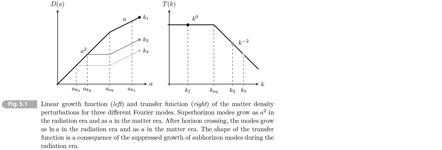
In the matter era the density contrast grows as 𝑎(𝑡) both inside and outside the horizon. For modes entering the horizon in the matter era the growth is therefore independent of scale. In contrast, in the radiation era, the perturbation s evolve very differently inside and outside the horizon. Subhorizon modes experience only logarithmic growth, while superhorizon modes grow as 𝑎2. Since the moment of horizon entry depends on the wavenumber of the mode 𝑘 = 𝑎𝐻, this leads to a 𝑘-dependent growth of the fluctuations. We describe this effect by so-called transfer function:
(5.67) 𝛵(𝑘) ≡ 𝐷+(𝑡𝑖)/𝐷+(𝑡) 𝛿(𝐤, 𝑡)/𝛿(𝐤, 𝑡𝑖),
where 𝐷+ is the scale-independent growth function. The function 𝛵(𝑘) captures all deviation in the evolution due to the scale-dependent growth in the radiation era. Because the evolution is isotropic, the transfer function depends only on the magnitude of the wavevector. The initial time 𝑡𝑖 is taken to be some time after inflation, when all modes of interest were still outside the horizon.
Let us denote by 𝑘eq ≡ (𝑎𝐻)eq that entered the horizon at the time of matter-radiation equality. This scale separates modes in the radiation era (𝑘 > 𝑘eq) from that in the matter era (𝑘 < 𝑘eq).
First, we consider long-wavelength modes with 𝑘 < 𝑘eq, like the mode 𝑘1, shown in Fig. 5.1. These modes were outside the horizon era and hence grow 𝛿 ~ 𝑎2 and in the matter era the growth slowed to 𝛿 ~ 𝑎. These considerations imply that
(5.68) 𝛿(𝐤, 𝑡) = (𝑎eq/𝑎𝑖)2 𝑎/𝑎eq 𝛿(𝐤, 𝑡𝑖) ≡ 𝐷+(𝑡)/𝐷+(𝑡𝑖) 𝛿(𝐤, 𝑡𝑖), for 𝑘 < 𝑘eq.
As expected the transfer function for mode entering the horizon during the matter era is trivial 𝛵(𝑘 < 𝑘eq) =1.
Next, we follow the evolution of short-wavelength modes with 𝑘 > 𝑘eq, like 𝑘2 and 𝑘3 in Fig. 5.1. These modes enter the horizon at time 𝑡𝑘 in the radiation era, Before horizon entry, the the modes grows as 𝛿 ~ 𝑎2, while after the horizon entry, the growth becomes logarithimic, 𝛿 ~ ln 𝑎. For simplicity, we will assume that 𝛿 ~ const, i.e. the growth has stopped completely. The modes start to grow again as 𝛿 ~ 𝑎 only after the universe has become matter dominated. We therefore get
(5.69) 𝛿(𝐤, 𝑡) = (𝑎𝑘/𝑎𝑖)2 𝑎/𝑎eq 𝛿(𝐤, 𝑡𝑖) = (𝑎𝑘/𝑎eq)2 × [𝑎eq/𝑎𝑖)2 𝑎/𝑎eq] 𝛿(𝐤, 𝑡𝑖), for 𝑘 > 𝑘eq,
where the term in the square brackets is the same 𝑘-independent factor as in (5.68). We see that the amplitude is suppressed by an additional factor of (𝑎𝑘/𝑎eq)2. Since (according to Friedmann equation) 𝐻 ∝ 𝑎2 in the radiation era, a mode with wavenumber 𝑘 enters the horizon at 𝑘 = (𝑎𝐻)𝑘 ∝ 1/𝑎𝑘.The suppression factor can therefore also be written as (𝑎𝑘/𝑎eq)2= (𝑘eq/𝑘)2 and the transfer function is 𝛵(𝑘 > 𝑘eq) = (𝑘eq/𝑘)2.
In summary, the results in (5.68) and (5.69) imply
(5.70) 𝛵(𝑘) ≈ { 1 𝑘 < 𝑘eq, (𝑘eq/𝑘)2 𝑘 > 𝑘eq.
Including the logarlithmic growth during the radiation era would give 𝛵(𝑘) ≈ (𝑘eq/𝑘)2 in (𝑘/𝑘eq) for 𝑘 > 𝑘eq. Our treatment has also ignored the effect of baryons on the thransfer function. In section 6.4.3 we will show that sound waves in the photon-baryon fluid before fluid decoupling lead to an oscillatory feature in the dark matter transfer function.
5.2 Statistical Properties
It is a crucial fact the large-scale structure in the universe isn't distributed randomey, but has interesting correlations between spatially separated points. A brief introduction to these correlations will be discussed.
5.3.1 Correlation Functions
By definition, the mean value of density perturbations is zero, ⟨𝛿⟩ = 0. The first nontrivial statistical measure of the density field (at a fixed time 𝑡) is therefore the two-point correlation function
(5.71) 𝜉(∣𝐱 - 𝐱'∣, 𝑡) ≡ ⟨𝛿(𝐱, 𝑡)𝛿(𝐱', 𝑡) ⟩ = ∫ 𝒟𝛿 𝚸∣𝛿∣ 𝛿(𝐱, 𝑡)𝛿(𝐱', 𝑡),
To avoid clutter, the time dependence will often be suppressed. The integral is functional integral over field configurations and 𝚸∣𝛿∣ is the probability of realizing some field configuration 𝛿(𝐱). The expected value ⟨∙ ∙ ∙⟩ denotes an ensemble average of stochastic process that created the random field 𝛿(e.g. quantum fluctuations during inflation; see Chapter 8). The homogeneity of the universe implies that the two-point function should be invariant under a translation of the spatial coordinates, i.e. it can only depend on the separation between the two points, 𝐱 - 𝐱'. Moreover, by isotropy the correlation function must be invariant under rotations and hence can only depend on the distance between the points, 𝑟 ≡ ∣𝐱 - 𝐱'∣. Equation (5.71) has a natural generalization to correlations between more than two points, but for now we will focus on the two-point function.
While the ensemble average is the natural object to compute from a theory of the initial conditions, it is not what we actually measure in the observations. The observed large-scale structure of the universe is a single realization of a random process. To relate these observations to our theoretical predictions, we assume ergodicity, which states that ensemble averages are equal to spatial averages as the volume become s infinitely large, For a Gaussian random field, ergodic behavior holds if 𝜉(𝑟) → 0 for 𝑟 → ∞. In that case, different parts of the universe can be viewed as different realizations of the underlying random process. The volume average therefore approximates the average over different members of ensemble. For example, galaxy surveys measure objects only out to a maximal redshift. The finite volume of the survey will introduce statistical fluctuations called sample variance. In CMB the volume is bounded by the size of the observable universe itself. The associated sample variance is then also called cosmic variance and arises because we only have one finite universe to observe.
Above we have seen that the Fourier modes of small fluctuations evolve independently. It is therefore very useful to define the two-point function in Fourier space
(5.72) ⟨𝛿(𝐤)𝛿*(𝐤')⟩ = ∫ 𝑑3𝑥𝑑3𝑥' 𝑒-𝑖𝐤⋅𝐱𝑒𝑖𝐤'⋅𝐱' ⟨𝛿(𝐱)𝛿(𝐱')⟩ = ∫ 𝑑3𝑥𝑑3𝑥' 𝑒-𝑖𝐤⋅𝐱𝑒𝑖(𝐤-𝐤')⋅𝐱' 𝜉(𝑟)
= (2π)3𝛿𝐷(𝐤 - 𝐤') ∫ 𝑑3𝑟 𝑒𝑖𝐤⋅𝐫 𝜉(𝑟) = (2π)3𝛿𝐷(𝐤 - 𝐤') 𝒫(𝑘),
[𝛿𝐷(𝐤 - 𝐤') ≡ 1/2π ∫-∞∞ 𝑒𝑖(𝐤-𝐤')⋅𝐱' 𝑑𝑥' { ∞, if 𝐤 = 𝐤'; 0, otherwise.]
where, in the second line, we introduced 𝐫 ≡ 𝐱 - 𝐱' and then performed the integral over 𝐱'. The fact that the result is proportional to the Dirac delta function 𝛿𝐷(𝐤 - 𝐤') is a consequence of translation invariance. The delta function implies that Fourier modes with different wavevectors are independent of each other. The function 𝒫(𝑘) is called the power spectrum and is the three-dimensional Fourier transform of the correlation function 𝜉(𝑟). Because of rotational invariance, the power spectrum depends only on the magnitude of the wavevector, 𝑘 ≡ ∣𝐤∣. Working in spherical polar coordinates, 𝐤 ⋅ 𝐫 = 𝑘𝑟 cos 𝜃 and the power spectrum can be written as
(5.73) 𝒫(𝑘) = ∫ 𝑑3𝑟 𝑒-𝑖𝐤⋅𝐫 𝜉(𝑟)
= ∫02π 𝑑𝜙 ∫-1+1 𝑑(cos 𝜃) ∫0∞ 𝑑𝑟 𝑟2 𝑒-𝑖𝑘𝑟 cos 𝜃 𝜉(𝑟)
= 2π ∫0∞ 2/𝑖𝑘𝑟 [𝑒𝑖𝑘𝑟 - 𝑒-𝑖𝑘𝑟] 𝜉(𝑟) = 4π/𝑘 ∫0∞ 𝑑𝑟 𝑟 sin(𝑘𝑟) 𝜉(𝑟).
While the correlation function 𝜉(𝑟) is natural object to consider in observations, the power spectrum 𝒫(𝑘) is easier to predict theoretically. The two are related by (5.73) and are therefore completely equivalent description of the statistics.
Exercise 5.5 Show that
(5.74) 𝜉(𝑟) = ∫ 𝑑𝑘/𝑘 𝑘3/2π2 𝒫(𝑘) 𝑗0(𝑘𝑟),
where 𝑗0(𝑥) = sin 𝑥/𝑥.
[Solution] The correlation function can be expressed as
(a) 𝜉(𝑟) = ⟨𝛿(𝐱)𝛿(𝐱')⟩ = ∫ (𝑑3𝑘 𝑑3𝑘')/(2π)6 ⟨𝛿(𝐤)𝛿*(𝐤')⟩ 𝑒𝑖𝐤⋅𝐱 𝑒𝑖𝐤'⋅𝐱'. [RE (5.14)]
Using the definition of the two-point function in Fourier space ⟨𝛿(𝐤)𝛿*(𝐤')⟩ = (2π)3 𝛿𝐷(𝐤 - 𝐤') 𝒫(𝑘)
(b) 𝜉(𝑟) = ∫ (𝑑3𝑘 𝑑3𝑘')/(2π)3 𝛿𝐷(𝐤 - 𝐤') 𝒫(𝑘) 𝑒𝑖𝐤⋅𝐱 𝑒𝑖𝐤'⋅𝐱' = ∫ 𝑑3𝑘/(2π)3 𝒫(𝑘) 𝑒𝑖𝐤⋅(𝐱 - 𝐱').
Going to polar coordinates, we find
(c) 𝜉(𝑟) = 1/(2π)3 ∫0∞ 𝑘2 𝑑𝑘 ∫02π 𝑑𝜙 ∫-1+1 𝑑(cos 𝜃) 𝒫(𝑘) 𝑒𝑖𝑘𝑟 cos 𝜃 = 1/4π2 ∫0∞ 𝑘2 𝑑𝑘 (𝑒𝑖𝑘𝑟 - 𝑒-𝑖𝑘𝑟)/𝑖𝑘𝑟 𝒫(𝑘)
= ∫0∞ 𝑑𝑘/𝑘 𝑘3/2π2 𝒫(𝑘) 𝑗0(𝑘𝑟). ▮
5.3.2 Gaussian Random Fields
For a Gaussian random field, the probability distribution 𝚸∣𝛿(𝐱)∣ is a Gaussian functional of 𝛿(𝐱). The probability deensity function for 𝑁 points in space, 𝐱1, ∙ ∙ ∙ , 𝐱𝑁, is then a multi-variate Gaussian
(5.75) 𝚸(𝛿1, ∙ ∙ ∙ , 𝛿𝑁) ∝1/√[det(𝜉𝑖𝑗) exp(-𝛿𝑖𝜉𝑖𝑗-1𝛿𝑗),
where 𝛿𝑖 ≡ 𝛿(𝐱𝑖) and 𝜉𝑖𝑗 ≡ 𝜉(∣𝐱𝑖 -𝐱𝑗∣). All 𝑁-point functions are then determined by a functional integral over 𝚸 and are fixed completely in terms of the two-point correlation function 𝜉(𝑟). As we will see in Chapter 8, inflation predicts that the initial conditions of the universe were described to a good approximation by a Gaussian random field. As long as the evolution is linear, the statistics remain Gaussian. The CMB probes the fluctuations mostly in the linear regime and they indeed look very Gaussian. So we will focus on Gaussian statistics of the two-point function (5.71) and the power spectrum (5.72).
At late times, however, structure formation is a highly nonlinear process and the probability distribution of the density field becomes non-Gaussian. A simple way to see this is to note that, by definition, the density contrast most satisfy 𝛿 > -1, while there is no such constraint for positive values of 𝛿. As 𝛿 becomes large, the probability distribution function must therefore asymmetric and non-Gaussian.
5.3.3 Harrison-Zel'dovich Spectrum
In Section 5.2.2 and 5.2.3 we described the linear evolution of a single Fourier mode of wavenumber 𝐤. Using these result, the power spectrum at time 𝑡 can be written as
(5.76) 𝒫(𝑘, 𝑡) = 𝛵2(𝑘) 𝐷+2(𝑡)/𝐷+2(𝑡𝑖) 𝒫(𝑘, 𝑡𝑖), [correction: 𝐷+(𝑡𝑖) → 𝐷+2(𝑡𝑖)]
where the transfer function satisfies 𝛵(𝑘 = 0) = 1. The Primordial power spectrum is often written in the following power law form
(5.77) 𝒫(𝑘, 𝑡𝑖) = 𝛢𝑘𝑛,
where 𝛢 and 𝑛 are constants. The exponent 𝑛 is called the spectral index. In 1970, well before inflation was introduced, it was argued by Harrion, Zel'dovich and Peebles that the initial perturbations of our universe are likely to have taken a power law form with the spectral index 𝑛 ≈ 1 [2-4]. This is now called the Harrison-Zel'dovich spectrum.
To see why the value 𝑛 ≈ 1 is special, we note that the Poisson equation ∇2𝛷 = 4π𝐺𝑎2𝜌̄ 𝛿, implies the following relation between the power spectra of 𝛷 and 𝛿:
(5.78) 𝒫𝛷(𝑘, 𝑡𝑖) ∝ 𝑘-4𝒫(𝑘, 𝑡𝑖) ∝ 𝑘𝑛-4.
Using (7.54), we furthermore see that the variance of the gravitational potential is
(5.79) 𝜎𝛷2 ≡ 𝜉𝛷(0) = ∫ 𝑑𝑘/𝑘 𝑘3/2π2 𝒫𝛷(𝑘, 𝑡𝑖) ≡ ∫ 𝑑𝑘/𝑘 ∆𝛷2(𝑘),
where we have introduced the dimensionless power spectrum
(5.80) ∆𝛷2(𝑘) ≡ 𝑘3/2π2 𝒫𝛷(𝑘, 𝑡𝑖) ∝ 𝑘𝑛-1.
For 𝑛 = 1, the dimensionless power spectrum of the gravitational potential therefore becomes 𝑘-independent, so that the variance receives equal contributions from every decade in 𝑘. This property of the field is called scale invariance.
Observations of the CMB have found that the spectral index is [5]
(5.81) 𝑛 = 0.9667 ± 0.0040.
The observed percent-level difference from the Harrison-Zel'dovich spectrum is precisely what is expected for fluctuations generated by inflation. As we will see Chapter 8, inflation predicts fluctuations that are naturally close to scale invariant because the inflationary dynamics is approximately time-translation invariant. However, we also know that inflation must end , so there has to be a small time dependence in the evolution. This translates into a small deviation from a perfectly scale-invariant spectrum.
1 As we will see in Chapter 6, on superhorizon scales, the Poisson equation depends on the choice of coordinates. Poisson equation to on superhorizon scales amount the so-called comoving gauge. We will denote density contrast in comoving gauge by ∆ not 𝛿.
|
|
|