|
김관석
|
2024-11-15 15:42:25, 조회수 : 105 |
- Download #1 : BC_7a.jpg (687.5 KB), Download : 0

7 Cosmic Microwave Background
Observations of CMB have played a pivotal role in the standard cosmological model. They provided the first evidence that the primordial fluctuations originated from quantum fluctuations during period of inflation. The fluctuations were captured when they still small and accurately described by linear perturbation theory. The physics of the CMB can be understood from first principle unlike the nonlinear structure formation in Chapter 5. Small fluctuations in the primordial plasma evolve under a well-defined set of equations, allowing very accurate predictions of the expected CMB temperature anisotropies.
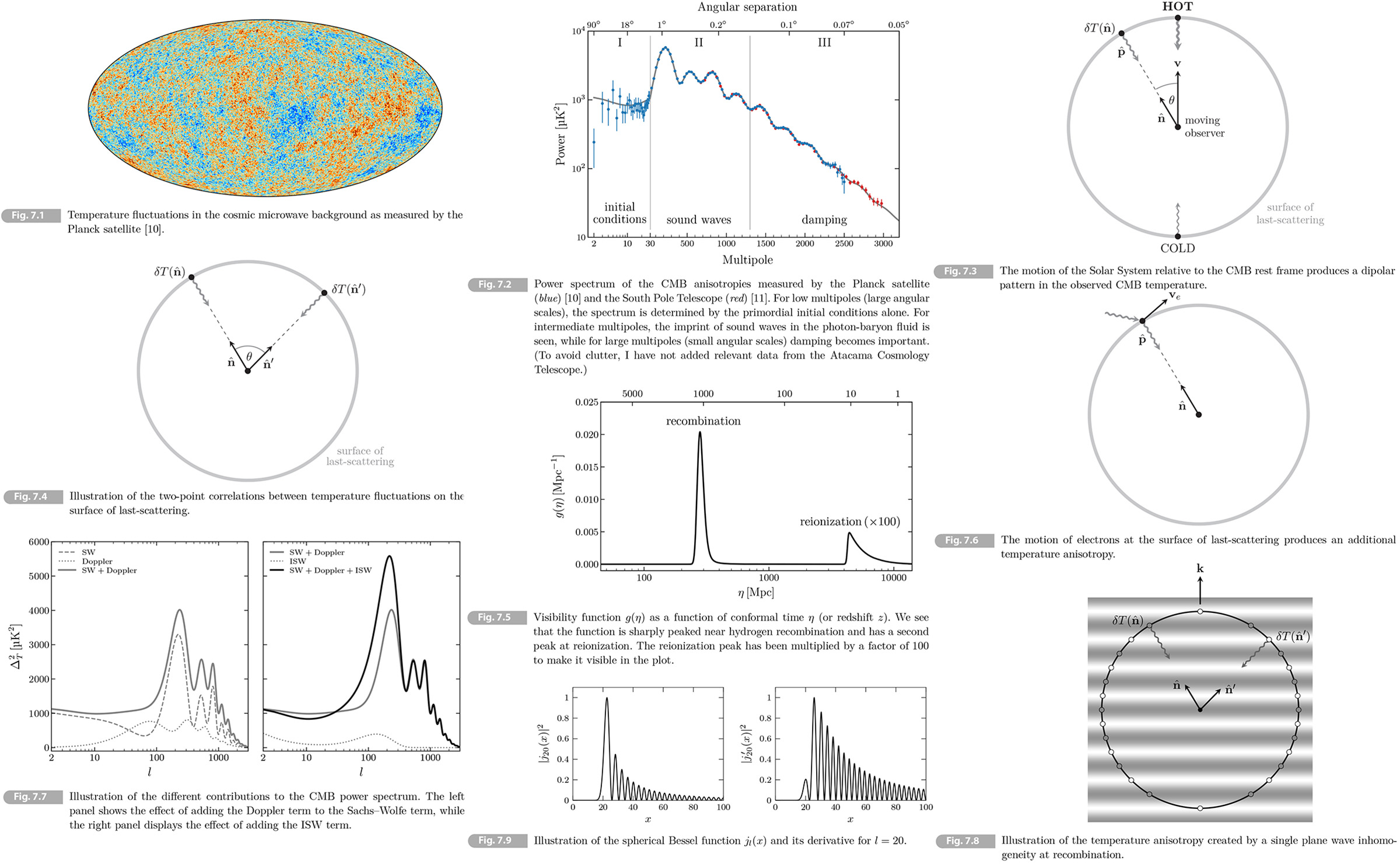
Fig. 7.1 is the stunning image of the universe in only 370,000 years old. It shows variations of intensity of the CMB photons at time of photon decoupling. The CMB temperature fluctuations are analyzed stastically as a function of their angular separation. The result is the angular power spectrum shown in Fig. 7.2 which shows a fit of the theoretical prediction for the CMB spectrum to data remarkably. It's usefule to separate them into three regimes as I, II and III:
• Region I: Large angle correlations are sourced by fluctuations that were still outside the horizon at recombination. These are a direct probe of the initial conditions.
• Region II: Perturbations with shorter wavelengths entered the horizon before recombination. Inside the horizon the perturbations in the tightly-coupled photon-baryon fluid propagate as sound waves supported by the large photon pressure. The oscillation frequency is a function of their wavelength, so that different modes are captured at different moments in their evolution at photon decoupling. This is the origin of the oscillatory pattern seen in the angular power spectrum.
• Region III: On small scales, the random diffusion of the photon has led to a damping of the eave amplitude. This suppresses the amplitude of the CMB power spectrum on small angular scales (large multipole moments).
The goal is to understand how the cosmological parameters determine the shape of the power spectrum, so that we can understand how the CMB measurements constrain these parameters. The evolution of fluctuations in a hydrodynamic approximation will be presented. This approximation works well, but breaks down below the mean free path of the photons. A fully self-consistent treatment of the CMB anisotropies by Boltzmann equation will be given in Appendix B.
7.1 Anisotropies in the First Light
The largest anisotropy in the CMB is a temperature dipole of magnitude 3.36 mK, which is due to the motion of the Solar system with respect to the CMB rest frame. As Problem 7.1 the motion creates a Doppler shift and hence a temperature anisotropy
(7.1) 𝛿𝛵(𝐧̂)/𝛵 = 𝐧̂ ⋅ 𝐯 = 𝑣 cos(𝜃),
where 𝐧̂ is a unit vector pointing in the observer's line of sight,which is the opposite to the momentum of the incoming radiation 𝐩̂ and 𝐯 is the velocity of the observer (see Fig. 7.3). The temperature is higher if we move toward the radiation (𝐧̂ ⋅ 𝐯 = 𝑣) and smaller if we move away from it (𝐧̂ ⋅ 𝐯 = -𝑣). Fitting this dipolar anisotropy to the data, we find 𝑣 = 368 km/s.2. After subtracting the dipole, we are left with the cosmological signal in Fig. 7.1.
7.1.1 Angular Power Spectrum
Let 𝛵(𝐧̂) ≡ 𝛵̄0[1 + 𝛩(𝐧̂)] be the measured CMB temperature in the direction 𝐧̂ in the sky, where 𝛵̄0 is the average CMB temperature today and we introduced the fractional temerature fluctuation 𝛩(𝐧̂) ≡ 𝛿𝛵(𝐧̂)/𝛵̄0. Comparing the temperature at two distinct 𝐧̂ and 𝐧̂ʹ (see Fig. 7.4) gives the two point correlation function
(7.2) 𝐶(𝜃) ≡ ⟨𝛩(𝐧̂)𝛩(𝐧̂ʹ)⟩,
where cos(𝜃) = 𝐧̂ ⋅ 𝐧̂ʹ. The angle bracket denote an average over an ensemble universe. Our universe is only one member of this ensemble, but we can estimate the ensemble average by dividing the CMB into independent patches and averaging over the correlations in each patch. For large-angle correlations, the number of independent patches is small and this estimate will have a large variance.
Given that we observe fluctuations on the spherical surface of last scattering, it is convenient to expand the temperature field in spherical harmonics
(7.3) 𝛩(𝐧̂) = ∑∞𝑙=2∑𝑙𝑚=-𝑙 𝑎𝑙𝑚𝑌𝑙𝑚(𝐧̂),
where the expansion coefficients 𝑎𝑙𝑚 are called multipole moments. A few relevant mathematical properties of the spherical harmonics are reviewed in Appendix D. There are various phase conventions for the 𝑌𝑙𝑚; We will adopt 𝑌*𝑙𝑚 = (-1)𝑚, so that 𝑎*𝑙𝑚 = (-1)𝑚𝑎*𝑙,-𝑚 for a real field 𝛩(𝐧̂). The two-point function of the multipole moments is defined as
(7.4) ⟨𝑎*𝑙𝑚𝑎*𝑙ʹ𝑚ʹ⟩ = 𝐶𝑙𝛿𝑙𝑙ʹ𝑚𝑚ʹ,
where 𝐶𝑙 is the angular power spectrum and the Kronecker deltas are a consequence of statistical isotropy. The angular power spectrum is the harmonic space equivalent of the two-point correlation function in real space. Substituting (7.3) into (7.2), we get
(7.5) 𝐶(𝜃) = ⟨𝛩(𝐧̂)𝛩(𝐧̂ʹ)⟩ = ∑𝑙𝑚∑𝑙ʹ𝑚ʹ⟨𝑎*𝑙𝑚𝑎*𝑙ʹ,𝑚ʹ⟩𝑌𝑙𝑚(𝐧̂)𝑌*𝑙ʹ𝑚ʹ(𝐧̂ʹ) = ∑𝑙𝐶𝑙∑𝑚𝑌𝑙𝑚(𝐧̂)𝑌*𝑙ʹ𝑚ʹ(𝐧̂ʹ) = ∑𝑙(2𝑙 + 1)/4π 𝐶𝑙𝑃𝑙(cos(𝜃)),
where 𝑃𝑙(cos(𝜃)) are Legendre polynomials (see Appendix D). Wee see that the moments of the angular power spectrum appear as coefficients in an expansion of 𝐶(𝜃) in terms of Legendre polynomials. Using the orthogonality of the Legendre polynomials, we can also write
(7.6) 𝐶𝑙 = 2π ∫1-1d cos(𝜃) 𝐶(𝜃)𝑃𝑙(cos(𝜃)).
The variance of the temperature anisotropy field is
(7.7) 𝐶0 = ∑𝑙(2𝑙 + 1)/4π 𝐶𝑙 ≈ ∫ d ln 𝑙 (2𝑙 + 1) 𝑙𝐶𝑙/4π ≈ ∫ d ln 𝑙 𝑙(𝑙 + 1)𝐶𝑙/2π,
where the final equality holds for 𝑙 ≫ 1. The power per logarithmic interval in 𝑙 is
(7.8) ∆2𝛵 ≡ 𝑙(𝑙 + 1)/2π 𝐶𝑙𝛵̄02.
We usually plot the CMB power spectrum as ∆2𝛵, which on large scales (small multiples) will be independent of 𝑙 if the primordial fluctuations are scale invariant (See Section 7.3.2). Note that our ∆2𝛵 is the same as 𝓓𝑙 in the Plank papers.
Finally we return to the cosmic variance. For fixed 𝑙, we have 2𝑙 + 1 different 𝑎𝑙𝑚's, allowing for 2𝑙 + 1 independent of 𝑙 independent estimates of the true 𝐶𝑙's. Imagine that we made a full-sky noise-free observation of the temperature field 𝛩(𝐧̂) and extracted its multipole moments 𝑎𝑙𝑚. An estimator for 𝐶𝑙 is
(7.9) 𝐶̂𝑙 ≡ 1/(2𝑙 + 1) ∑𝑚∣𝑎𝑙𝑚∣2.
This estimator is unbiased in the sense that ⟨𝐶̂𝑙⟩ = 𝐶𝑙. However, the estimator has a nonzero variance corresponding to an irreducible error in our determination of the true power spectrum
(7.10) ∆𝐶𝑙/𝐶𝑙 ≡ √⟨(𝐶𝑙 - 𝐶̂𝑙)⟩/𝐶𝑙 = √[2/(2𝑙 + 1)].
This cosmic variance is largest for small 𝑙, corresponding to large scales. this explain why the error bars in Fig. 7.2, which contain both cosmic variance and instrumental noise, are largest for small multipoles. Curren measurements from Plank are dominated by cosmic variance up to 𝑙 ~ 2000.
Exercise 7.1 Use Wick's theorem, to derive (7.10)
(7.11) ⟨𝑎𝑙𝑚𝑎*𝑙𝑚𝑎𝑙𝑚ʹ𝑎*𝑙𝑚ʹ ⟩ = ⟨𝑎𝑙𝑚𝑎*𝑙𝑚⟩⟨𝑎𝑙𝑚ʹ𝑎*𝑙𝑚ʹ⟩ + ⟨𝑎𝑙𝑚𝑎*𝑙𝑚ʹ⟩ + ⟨𝑎𝑙𝑚ʹ𝑎*𝑙𝑚ʹ⟩⟨𝑎*𝑙𝑚𝑎𝑙𝑚ʹ⟩.
[Solution] Using ⟨𝐶̂𝑙⟩ = 𝐶𝑙 and Wick's theorem
(a) ∆𝐶𝑙2 = ⟨(𝐶̂𝑙 - 𝐶𝑙)2⟩ = ⟨𝐶̂𝑙𝐶̂𝑙 - 2𝐶𝑙⟨𝐶̂𝑙⟩ + 𝐶𝑙2 = 1/(2𝑙 + 1)2 ∑𝑚𝑚ʹ⟨𝑎𝑙𝑚𝑎*𝑙𝑚𝑎𝑙𝑚ʹ𝑎*𝑙𝑚ʹ⟩ - 𝐶𝑙2.
(b) ∆𝐶𝑙2 = 1/(2𝑙 + 1)2 ∑𝑚𝑚ʹ(⟨𝑎𝑙𝑚𝑎𝑙𝑚ʹ⟩⟨𝑎*𝑙𝑚𝑎*𝑙𝑚ʹ⟩ + ⟨𝑎𝑙𝑚𝑎*𝑙𝑚ʹ⟩⟨𝑎*𝑙𝑚𝑎𝑙𝑚ʹ⟩)
(c) ⟨𝑎𝑙𝑚𝑎𝑙𝑚ʹ⟩ = (-1)𝑚ʹ⟨𝑎𝑙𝑚𝑎*𝑙,-𝑚ʹ⟩ = (-1)𝑚ʹ𝐶𝑙𝛿𝑚,-𝑚ʹ, ⟨𝑎*𝑙𝑚𝑎*𝑙𝑚ʹ⟩ = (-1)𝑚ʹ⟨𝑎*𝑙𝑚𝑎𝑙,-𝑚ʹ⟩ = (-1)𝑚ʹ𝐶𝑙𝛿𝑚,-𝑚ʹ,
⟨𝑎𝑙𝑚𝑎*𝑙𝑚ʹ⟩ = 𝐶𝑙𝛿𝑚,𝑚ʹ, ⟨𝑎*𝑙𝑚𝑎𝑙𝑚ʹ⟩ = 𝐶𝑙𝛿𝑚,𝑚ʹ. ⇒
(c) ∆𝐶𝑙2 = 2/(2𝑙 + 1)2 𝐶𝑙2. ⇒ ∆𝐶𝑙/𝐶𝑙 = √[2/(2𝑙 + 1)]. ▮
7.1.2 A Road Map
Our main goal is now to understand how the observed power spectrum of CMB anisotropies is related to the spectrum of initial curvature perturbation:
∆𝓡2(𝑘) ≡ 𝑘3/2π2 𝒫𝓡(𝑘) → 𝐶𝑙 = 4π ∫ d ln 𝑘 𝛩𝑙2(𝑘)∆𝓡2(𝑘)
The transfer function 𝛩𝑙(𝑘) that maps ∆𝓡2(𝑘) to 𝐶1 captures the evolution of the fluctuation in the primordial plasma, the free streaming of the photon after decoupling and the projection of the anisotropies onto the sky.
𝓡(0,𝑘) evolution (§7.4)→ [𝛿𝛾, 𝛹, 𝑣𝑏]𝜂* free streaming (§7.2); projection (§7.3)→ 𝛿𝛵(𝐧̂)
where 𝓡 is the initial curvature perturbations, which requires us to follow the evolution of coupled perturbations from early times until decoupling and 𝛿𝛵(𝐧̂) is fluctuations on the surface of last-scattering. The CMB anisotropies depends on the fluctuation in the photon density (𝛿𝛾), the gravitational potential (𝛹) and the baryon density (𝑣𝑏) at the time of decoupling (𝜂*). We will explain that the projection of these inhomogeneities onto the observer's sky leads to nontrivial angular variation. Since the evolution is linear, we can study each Fourier mode separately, and the final anisotropy spectrum is obtained by summing over many Fourier modes weighted by the spectrum of the initial conditions.
7.2 Photons in a Clumpy Universe
We begin with the free streaming of the photon after decoupling. As the photons travel through the inhomogeneous universe they gain and lose their energy, which will affect the observed temperature anisotropies.
7.2.1 Gravitational redshift
The evolution of the photons after decoupling is governed by the geodesic equation (see Chapter 2 and Appendix A)
(7.12) d𝑃𝜇/d𝜆 = -𝛤𝜇𝜈𝜌𝑃𝜈𝑃𝜌,
where 𝑃𝜇 = d𝑥𝜇/d𝜆. We will work in Newtonian gauge as
(7.13) d𝑠2 = 𝑎2(𝜂)[-(1 + 2𝛹)d𝜂2 + (1 - 2𝛷)𝛿𝑖𝑗d𝑥𝑖d𝑦𝑗].
The case of tensor perturbations will be explored in Problem 7.6.
(7.14) d𝑃𝜇/d𝜆 = d𝜂/d𝜆 d𝑃𝜇/d𝜂 = 𝑃0 d𝑃𝜇/d𝜂.
To determine the evolution of the photon energy, we consider the time component of (7.12):
(7.15) d𝑃𝜇/d𝜂 = -𝛤0𝜈𝜌 𝑃𝜈𝑃𝜌/𝑃0 = -𝛤000𝑃0 - 2𝛤00𝑖𝑃𝑖 - 𝛤0𝑖𝑗 𝑃𝑖𝑃𝑗/𝑃0
= -(𝓗 + 𝛹ʹ)𝑃0 - 2∂𝑖𝛹𝑃𝑖 - [𝓗 - 𝛷ʹ - 2𝓗(𝛷 + 𝛹)]𝛿𝑖𝑗 𝑃𝑖𝑃𝑗/𝑃0.
The 4-momentum components 𝑃𝜇 = (𝑃0, 𝑃𝑖) are defined in the coordinate frame, while what an observer actually measures as the photon energy and momentum are components 𝑃𝜇̂ = (𝑃0, 𝑃𝑖̂) in their local inertial frame. to relate these we use that
(7.16) 𝜂𝜇̂𝜈̂𝑃𝜇̂𝑃𝜈̂ = 𝑔𝜇𝜈𝑃𝜇𝑃𝜈, -𝛦2 + 𝛿𝑖𝑗𝑃𝑖𝑃𝑗 = 𝑔00(𝑃0)2 + 𝑔𝑖𝑗𝑃𝑖𝑃𝑗.
The energy and momentum in the local inertial frame can therefore be written as3 [RE 2.55-6]
(7.17) 𝐸 = √-𝑔00 𝑃0, 𝑝2 ≡ 𝑔𝑖𝑗𝑃𝑖𝑃𝑗 = 𝛿𝑖𝑗𝑃𝑖̂𝑃𝑗̂, and hence we have [using Taylor series]
(7.18) 𝑃0 = 𝐸/√-𝑔00 = 𝐸/√[𝑎2(1 + 2𝛹)] = 𝐸/𝑎 (1 - 𝛹), 𝑃𝑖 = 𝐸/√[𝑎2(1 - 2𝛷)𝑝̂𝑖] = 𝐸/𝑎 (1 + 𝛷)𝑝̂𝑖,
where 𝑝̂𝑖 is the unit vector in the photon's direction of propagation. Substituting (7.18) into (7.15), we get
(7.19) d/d𝜂 [𝐸/𝑎 (1 - 𝛹)] = -(𝓗 + 𝛹ʹ)𝐸/𝑎 (1 - 𝛹) - 2∂𝑖𝛹 𝐸/𝑎 (1 + 𝛷)𝑝̂𝑖 - [𝓗 - 𝛷ʹ - 2𝓗(𝛷 + 𝛹)] 𝐸/𝑎 (1 + 𝛷)2/(1 - 𝛹),
which, at first order cleans up
(7.20) 1/𝐸 d𝐸/d𝜂 = -𝓗 + 𝛷ʹ - 𝑝̂𝑖∂𝑖𝛹,
where we used that
(7.21) d𝛹/d𝜂 = ∂𝛹/∂𝜂 + d𝑥𝑖/d𝜂 ∂𝑖𝛹 ≡ 𝛹ʹ + 𝑝̂𝑖∂𝑖𝛹.
The right-hand side of (7.20) has a clear physical interpretation: The first term describes the redshifting of photo energy due to the expansion of the universe, 𝐸 ∝ 𝑎-1. The metric potential 𝛷 can be viewed as a local perturbation of the scale factor, 𝑎˜(𝜂, 𝐱) = 𝑎(𝜂)(1 - 𝛷). The 𝛷ʹ term in (7.20) simply captures the fact that the photon energy now decrease as 𝐸 ∝ 𝑎˜-1. The third term proportional to ∂𝑖𝛹 describes gravitational redshift (or blueshift) as the photon travels out of (or falls into) a gravitational well. Using (7.21) we cab write
(7.22) 𝑝̂𝑖∂𝑖𝛹 = d𝛹/d𝜂 - ∂𝛹/∂𝜂 ≡ d𝛹/d𝜂 - 𝛹ʹ, so that (7.20) becomes
(7.23) d ln(𝑎𝐸)/d𝜂 = -d𝛹/d𝜂 + 𝛷ʹ + 𝛹ʹ.
This equation determines how he inhomogeneities in he spacetime affect the photon energy, beyond the usual redshifting due to the expansion of the universe.
7.2.2 Line-of-Sight Solution
By integrating the geodesic equation (7.23) we can relate the energy of CMB photon at decoupling to its energy today, when it enters our detectors. We will assume that recombination was nearly instanteneous so that all photons were released at the same time 𝜂*. This assumption is justified by the visibility function (see Section 3.2.5), which we define in terms of conformal time:
(7.24) 𝑔(𝜂) ≡ d/d𝜂 𝑒-𝜏 = -𝜏ʹ𝑒-𝜏,
where 𝜏 is the optical depth. The visibility function describes the probability that a photon last scattered in the interval [𝜂, 𝜂 + d𝜂]. Fig. 7.5 shows that the visibility function is sharply peaked at 𝜂* ≈ 373 000 yrs (or 𝑧* ≈ 1090), the moment of last scattering.
Letting our location be the origin of coordinates, 𝐱0 ≡ 0, the photons in a direction 𝐧̂ were emitted at the point 𝐱* ≡ 𝜒*𝐧̂, where 𝜒* = 𝜂0 - 𝜂* is the distance to the last-scattering surface (in a flat universe). Integrating (7.23) from the time of emission 𝜂* to the time of observation 𝜂0, we get
(7.25) ln(𝑎𝐸)0 = ln(𝑎𝐸)* - (𝛹0 - 𝛹*) + ∫𝜂0𝜂*d𝜂 (𝛷ʹ + 𝛹ʹ).
After decoupling, the photon distribution function maintains the same shape, because all photons simply move along geodesics. Since the Bose-Einstein distribution is a function of 𝛦/𝛵, this means 𝛵 ∝ 𝛦 (see Chapter 3). So we can relate
the perturbed photon energy to the temperature anisotropy:
(7.26) 𝑎𝐸 ∝𝑎𝛵̄ (1 + 𝛿𝛵/𝛵̄),
where 𝛵̄ is the mean temperature. Taylor expanding the logaritims in (7.25) to the first order [ln(1 + 𝑥)] ≈ 𝑥, (𝑥 = 0).] and since 𝑎0𝛵̄0 = 𝑎*𝛵̄*, we find
(7.27) 𝛿𝛵/𝛵̄∣0 = 𝛿𝛵/𝛵̄∣* + 𝛹* + ∫𝜂0𝜂*d𝜂 (𝛷ʹ + 𝛹ʹ),
where we drop 𝛹0 since it only contribute to the 𝑙 = 0 monopole and is hence unobservable. [verification needed]
7.2.3 Fluctuations at Last-Scattering
We see from (7.27) that the observed temperature fluctuation today, 𝛿𝛵0, depend on the intrinsic temperature fluctuations at the moment of the last-scattering, 𝛿𝛵*. The latter have two distinct sources:
• First, there are fluctuations due to photon density at recombination; since 𝜌𝛾 ∝𝛵4 [RE (3.35)], 𝛿𝛵/𝛵 ⊂ 𝛿𝛾/4. So the regions of enhanced photon density regions are slightly hotter and vice versa.
• Second, there are there are fluctuations due to bulk velocity of the electrons at recombination. When the photons scatter off these electrons receive an additional Doppler shift of the form 𝛿𝛵/𝛵 ⊂ 𝐩̂ ⋅ 𝐯𝑒, where 𝐩̂ is a unit vector associated with the momentum of the scattered photon (see Fig. 7.6).4 A formal derivation using Boltzmann equation will be in Appendix B. Similarly with (7.1) the Doppler-induced temperature anisotropy due to our motion relative to the CMB frame.
Since 𝐩̂ = -𝐧̂ and the electrons are strongly interacting with the baryons, we can use 𝐯𝑒 = 𝐯𝑏 and write 𝛿𝛵/𝛵 ⊂ -𝐧̂ ⋅ 𝐯𝑏. Combing two sources we get
(7.28) 𝛿𝛵/𝛵̄̄∣* = (1/4 𝛿𝛾 - 𝐧̂ ⋅ 𝐯𝑏)*,
where * indicates that a quantity is evaluated at 𝜂* and the position 𝐱* on the surface of last-scattering.
(7.29) 𝛿𝛵/𝛵̄̄ (𝐧̂) = (1/4 𝛿𝛾 + 𝛹)*[← SW] - (𝐧̂ ⋅ 𝐯𝑏)*[← Doppler] + ∫𝜂0𝜂* d𝜂 (𝛷ʹ + 𝛹ʹ)[← ISW].
where we dropped the subscript 0 on the observed 𝛿𝛵/𝛵̄̄. The answer in (7.29) can be separated into three contributions:
• SW The first term is the so-called Sachs-Wolfe term [8]. It contains the intrinsic temperature fluctuations associated to the photon density fluctuations at last-scattering, 𝛿𝛾/4 with the induced temperature perturbation 𝛹* arising from the the gravitational redshift of the photons. In our conventions the negative 𝛹* leads to a temperature decrement, as expected since a photon loses energy when climbing out of a potential well.
• Doppler The Doppler term that we discussed before. Since the baryon velocity vanishes on superhorizon scales. We will find that the oscillations in the Doppler term are out of phase with the oscillations in the Sachs-Wolfe term, so that adding the Doppler contribution reduces the contrast between the peaks and troughs in the spectrum (see the left panel of Fig. 7.7.
• ISW The last term describes the additional gravitational redshift due to the evolution of the metric potentials along the line-of-sight. We call this the integrated Sachs-Wolfe (ISW) effect. A nonzero ISW effect requires that potential changes with time. At early times the residual amount of radiation gives 𝛷ʹ ≠ 0, which results in a nonzero early ISW effect. Adding this contribution raises the height of the first peak of the spectrum (see the right panel of Fig. 7.7). Similarly, at late times, dark energy becomes relevant, leading to a late ISW effect, which adds power for low 𝑙.
7.3 Anisotropies from Inhomogeneities
The line-sight-solution (7.29) shows how the observed CMB temperature fluctuations in a given direction are related to fluctuations at the surface of lass-scattering. In this section how the inhomogeneities in the primordial plasma give rise to correlations between the temperatures in different directions.
7.3.1 Spatial-to-Angular Projection
The evolution of the primordial fluctuations is best studied in Fourier space because of its linearity. Fig. 7.8 shows how a single Fourier mode cause angular variations in the CMB temperature. Let us for a moment ignore the ISW contribution.The temperature fluctuation in 𝐧̂ is then directly related to those at the point 𝐱* = 𝜒*𝐧̂ on the surface of last scattering. For scalar fluctuation, we have 𝐯𝑏 = 𝑖𝐤̂𝑣𝑏 and hence the (7.29) can be written as
(7.30) 𝛩(𝐧̂) = 𝛿𝛵/𝛵̄̄ (𝐧̂) = { d3𝑘/(2π)3 𝑒𝑖𝐤⋅(𝜒*𝐧̂) [𝐹(𝜂*, 𝐤) - 𝑖(𝐤̂ ⋅ 𝐧̂)𝐺(𝜂*, 𝐤)],
where 𝐹 ≡ 1/4 𝛿𝛾 + 𝛹 and 𝐺 ≡ 𝑣𝑏. Since the evolution is linear, it's convenient to factor out the initial curvature perturbation 𝓡𝑖(𝐤) ≡ 𝓡(0, 𝐤) and write
(7.31) 𝛩(𝐧̂) = 𝛿𝛵/𝛵̄̄ (𝐧̂) = { d3𝑘/(2π)3 𝑒𝑖𝐤⋅(𝜒*𝐧̂) [𝐹*(𝑘) - 𝑖(𝐤̂ ⋅ 𝐧̂)𝐺*(𝑘)]𝓡𝑖(𝐤),
where 𝐹*(𝑘) ≡ 𝐹(𝜂*, 𝐤) /𝓡𝑖(𝐤) and 𝐺*(𝑘) ≡ 𝐺(𝜂*, 𝐤)/𝓡𝑖(𝐤) are the transfer functions for the SW and Doppler terms. Note that these transfer functions only depend on 𝑘 ≡ ∣𝐤∣, while the initial perturbations are a function of its direction. We then use the Legendre expansion of the exponential
(7.32) 𝑒𝑖𝐤⋅(𝜒*𝐧̂) = ∑𝑙𝑖𝑙(2𝑙 + 1)𝑗𝑙𝑃𝑙(𝐤̂ ⋅ 𝐧̂),
where 𝑗𝑙 are the spherical Bessel functions (see Appendix D). The factor of 𝑖(𝐤̂ ⋅ 𝐧̂) of Doppler term leads to
(7.33) 𝑖(𝐤̂ ⋅ 𝐧̂)𝑒𝑖𝜒*𝐤⋅𝐧̂ = d/d(𝑘𝜒*) 𝑒𝑖(𝑘𝜒*)𝐤̂⋅𝐧̂ = ∑𝑙𝑖𝑙(2𝑙 + 1)𝑗𝑙ʹ(𝑘𝜒*)𝑃𝑙(𝐤̂ ⋅ 𝐧̂),
where the prime denote a derivative with respect to the argument of the spherical Bessel function. Substituting (7.32) and (7.33) into (7.31) we get
(7.34) 𝛩(𝐧̂) = ∑𝑙𝑖𝑙(2𝑙 + 1) ∫ d3𝑘/(2π)3 𝛩𝑙(𝑘)𝓡𝑖(𝐤)𝑃𝑙(𝐤̂ ⋅ 𝐧̂),
where we defined the transfer function
(7.35) 𝛩𝑙(𝑘) ≡ 𝐹*(𝑘)𝑗𝑙(𝑘𝜒*) - 𝐺*(𝑘)𝑗𝑙ʹ(𝑘𝜒*).
Inserting (7.34) into the two-point function (7.2) and using
(7.36-8) ⟨𝓡𝑖(𝐤)𝓡𝑖(𝐤ʹ)⟩ = 2π2/𝑘3 ∆𝓡2(𝑘)(2π)3𝛿𝐷(𝐤 + 𝐤ʹ), 𝑃𝑙(𝐤̂ ⋅ 𝐧̂) = (-1)𝑙𝑃𝑙(𝐤̂ ⋅ 𝐧̂), ∫ d𝐤̂ 𝑃𝑙(𝐤̂ ⋅ 𝐧̂)𝑃𝑙ʹ(𝐤̂ ⋅ 𝐧̂ʹ) = 4π/(2𝑙 + 1) 𝑃𝑙(𝐧̂ ⋅ 𝐧̂ʹ)𝛿𝑙𝑙ʹ,
we find
(7.39) ⟨𝛩(𝐧̂)𝛩(𝐧̂ʹ)⟩ = ∑𝑙 (2𝑙 + 1)/4π [4π ∫ d ln 𝑘 𝛩𝑙2(𝑘)∆𝓡2(𝑘)]𝑃𝑙(𝐧̂ ⋅ 𝐧̂ʹ).
Comparing this to (7.5), we identify the angular power spectrum as
(7.40) 𝐶𝑙 = 4π ∫ d ln 𝑘 𝛩𝑙2(𝑘)∆𝓡2(𝑘).
We see that the CMB power spectrum is determined by the power spectrum of the primordial curvature perturbations, ∆𝓡2(𝑘), and the transfer function 𝛩𝑙(𝑘). The latter describes both the evolution until decoupling and the projection onto the surface of last-scattering.
Exercise 7.2 Using the addition theorem
(7.41) 𝑃𝑙(𝐤̂ ⋅ 𝐧̂) = ∑∣𝑚∣≤𝑙 4π/(2𝑙 + 1) 𝑌*𝑙𝑚(𝐤̂)𝑌𝑙𝑚(𝐧̂),
show that the line-of-sight solution (7.34) can be written in the form (7.3) with
(7.42) 𝑎𝑙𝑚 = 4π𝑖𝑙 ∫ d3𝑘/(2π)3 𝛩𝑙(𝑘)𝓡𝑖(𝐤) 𝑌𝑙𝑚*(𝐤̂).
Show that substituting this into (7.4) gives the result in (7.40).
[Solution] Substituting (7.41) into (7.34) gives
(a) 𝛩(𝐧̂) = ∑𝑙 𝑖𝑙(2𝑙 + 1) ∫ d3𝑘/(2π)3 𝛩𝑙(𝑘)𝓡𝑖(𝐤)∑∣𝑚∣≤𝑙 4π/(2𝑙 + 1) 𝑌*𝑙𝑚(𝐤̂)𝑌𝑙𝑚(𝐧̂) = ∑𝑙𝑚[4π𝑖𝑙 ∫ d3𝑘/(2π)3 𝛩𝑙(𝑘)𝓡𝑖𝑌*𝑙𝑚(𝐤̂)]𝑌𝑙𝑚(𝐧̂),
Since 𝛩(𝐧̂) = ∑∞𝑙=2∑𝑙𝑚=-𝑙 𝑎𝑙𝑚𝑌𝑙𝑚(𝐧̂) in (7.3) we know
(b) 𝑎𝑙𝑚 = 4π𝑖𝑙 ∫ d3𝑘/(2π)3 𝛩𝑙(𝑘)𝓡𝑖(𝐤)𝑌*𝑙𝑚(𝐤̂).
Since ⟨𝑎*𝑙𝑚𝑎*𝑙ʹ𝑚ʹ⟩ = 𝐶𝑙𝛿𝑙𝑙ʹ𝑚𝑚ʹ in (7.4)
(c) ⟨𝑎*𝑙𝑚𝑎*𝑙ʹ𝑚ʹ⟩ = (4π)2𝑖𝑙-𝑙ʹ ∫ d3𝑘/(2π)3 ∫ d3𝑘ʹ/(2π)3 𝛩𝑙(𝑘)𝛩*𝑙(𝑘ʹ)⟨𝓡𝑖(𝐤)𝓡*𝑖(𝐤)⟩𝑌*𝑙𝑚(𝐤̂)𝑌𝑙ʹ𝑚ʹ(𝐤̂ʹ)
= (4π)2𝑖𝑙-𝑙ʹ ∫ d3𝑘/(2π)3 𝛩𝑙2 2π3/𝑘3 ∆𝓡(𝑘) 𝑌*𝑙𝑚(𝐤̂)𝑌𝑙ʹ𝑚ʹ(𝐤̂ʹ) = 4π ∫ d ln 𝑘 𝛩𝑙2(𝑘)∆𝓡2(𝑘) 𝛿𝑙𝑙ʹ𝛿𝑚𝑚ʹ ⇒
(d) 𝐶𝑙 = 4π ∫ d ln 𝑘 𝛩𝑙2(𝑘)∆𝓡2(𝑘). ▮
Including the ISW contribution, and repeating the same step, we find that the complete transfer function is
(7.43) 𝛩𝑙(𝑘) = 𝐹*(𝑘)𝑗𝑙(𝑘𝜒*) - 𝐺*(𝑘)𝑗𝑙ʹ(𝑘𝜒*) + ∫𝜂0𝜂*d𝜂 (𝛷ʹ + 𝛹ʹ)𝑗𝑙(𝑘𝜒),
where 𝜒(𝜂) = 𝜂0 - 𝜂. Substituting (7.43) into (7.40), in principle leads to six terms: the power spectrum, 𝐶𝑙SW, that of Doppler term, 𝐶𝑙D, that of the ISW term, 𝐶𝑙ISW, and three cross spectra. In practice, the cross spectra are small, although the cross relation between the SW and ISW terms plays a non-negligible role in the height of the first peak.
7.3.2 Large Scales: Sachs-Wolfe Effect
The low multipole of the CMB spectrum (𝑙 < 100) are created by superhorizon fluctuations at recombination. From Fig. 7.7 we see that this regime is dominated by the Sachs-Wolfe term. Let us evaluate it for adiabatic initial conditions.
Since decoupling ocuurs during the matter era, the superhorizon limit of the fluctuation implies -2𝛹 ≈ -2𝛷 ≈ 𝛿 = 𝛿𝑚 = 3/4 𝛿𝛾 and the observed MB temperature fluctuation on large scale are
(7.44) 𝛩(𝐧̂) ≈ (1/4 𝛿𝛾 + 𝛹)* = 1/3 𝛹* = 1/5 𝓡𝑖,
where te final equality follows from (6.155). Two points are worth noting: First since there has been no evolution on large scales, this limits of the CMB spectrum directly probes the initial conditions. Second, the gravitational redshift has won over the intrinsic temperature fluctuations. This means that an overdensity at last-sccattering (𝛿𝛾,* > 0), corresponding to a potential well (𝛹* < 0), leads to a cold spot in the CMB map (𝛩 < 0). Conversely a hot spot corresponds to an underdensity at last scattering.
The transfer function (7.43) for large-scale Sachs-Wolfe term then simply is
(7.45) 𝛩𝑙SW(𝑘) = 1/5 𝑗𝑙(𝑘𝜒*).
and the power spectrum (7.40) becomes
(7.46) 𝐶𝑙SW = 4π/25 ∫∞0 d ln 𝑘 ∆𝓡2(𝑘)𝑗𝑙2(𝑘𝜒*).
For a primordial spectrum of a power law form ∆𝓡2(𝑘) = 𝛢𝑠(𝑘/𝑘0)𝑛𝑠 - 1, the integral can be evaluated analytically and we find
(7.47) 𝐶𝑙SW = 4π/25 𝛢𝑠(𝑘0𝜒*)1 - 𝑛𝑠2𝑛𝑠 - 4π 𝛤(3 - 𝑛𝑠)/𝛤2(4 - 𝑛𝑠/2) 𝛤[𝑙 + (𝑛𝑠 - 1)/2]/𝛤[𝑙 + 2 - (𝑛𝑠 - 1)/2].
For 𝑛𝑠 = 1 the first ratio of gamma functions becomes 𝛤(2)/𝛤2(3/2) = 4/π,[verification needed] while the second ratio is [𝑙(𝑙 + 1)]-1.[verification needed] Moreover the scale dependence from (𝑘0𝜒*)1 - 𝑛𝑠 disappears, as expected for a spectrum with no intrinsic scale, and the power spectrum becomes
(7.48) 𝑙(𝑙 + 1)/2π 𝐶𝑙SW = 𝛢𝑠/25.
We see that a scale-invariant primordial spectrum 𝑘3𝒫𝓡(𝑘) = const, corresponds to the combination 𝑙(𝑙 + 1)𝐶𝑙 being a constant, independent of the multipole moment 𝑙. The amplitude of large-scale CMB spectrum is a direct measure of the amplitude 𝛢𝑠.
7.3.3 Small Scales: Sound waves
The larger multipoles (𝑙 > 100) are sourced by small-scale fluctuations on sub-Hubble scales. Here we just briefly comment on the projection effect for these scales.
For large values of 𝑙, the spherical Bessel function 𝑗𝑙(𝑥) is peaked near 𝑥 ≈ 𝑙 (cf. Fig. 7.9) and acts like a delta function in the integral (7.40). The derivative 𝑗𝑙ʹ is not as sharply peaked at 𝑥 ≈ 𝑙, so the projection from wavenumber 𝑘 to multipole 𝑙 is less sharp for Doppler term.5 We will indicate this by writing 𝑥 ~ 𝑙 rather than 𝑥 ≈ 𝑙. Therefore we have
(7.49) 𝑙(𝑙 + 1)/2π 𝐶𝑙SW ~ 𝐹*2(𝑘)∆𝓡2(𝑘)∣𝑘≈𝑙/𝜒*,
(7.50) 𝑙(𝑙 + 1)/2π 𝐶𝑙D ~ 𝐺*2(𝑘)∆𝓡2(𝑘)∣𝑘~𝑙/𝜒*,
where 𝐹*(𝑘) and 𝐺*(𝑘) are the transfer functions defined in (7.31), which is derived more rigorously in Exercise 7.3. For a scale-invariant initial conditions, ∆𝓡2(𝑘) = const, 𝐶𝑙SW and 𝐶𝑙D are determined simply by the squares of the transfer functions at 𝑘 = 𝑙/𝜒*. Oscillations in 𝑘become oscillations in 𝑙.
Exercise 7.3 For large 𝑙, the sperical Bessel functions can be approximated as
(7.51) 𝑗𝑙(𝑥) → { cos(𝑏)cos[𝜈(tan(𝑏) - 𝑏) - π/4]/𝜈√(sin(𝑏) 𝑥 > 𝜈; 0 𝑥 < 𝜈,
where 𝜈 ≡ 𝑙 + 1/2 and cos(𝑏) ≡ 𝜈/𝑥, with 0 ≤ 𝑏 ≤ π/2. Use this to show the following equations can be written
(7.52) 𝑙(𝑙 + 1)/2π 𝐶𝑙SW = ∫∞1 d𝛽/𝛽2√(𝛽2 - 1) 𝐹*2(𝑙𝛽/𝜒*)∆𝓡2(𝑙𝛽/𝜒*),
(7.53) 𝑙(𝑙 + 1)/2π 𝐶𝑙D = ∫∞1 d𝛽/𝛽2√(𝛽2 - 1) 𝐺*2(𝑙𝛽/𝜒*)∆𝓡2(𝑙𝛽/𝜒*),
where we see explicitly that the intergrand of the Doppler contribution vanishes for 𝛽 = 1. Given the transfer functions, these integrals are easy to evaluate numerically. Most of the contribution comes from 𝛽 ~ 1, so the intergrals can be performed with a finite cutoff, say 𝛽 = 5, without losing much accuracy [Weinberg].[verification needed]
2 The inferred speed has three components: (1) The orbital velocity of the Solar system with respect to the center of our Galaxy; (2)the velocity of our Galaxy with respect to the center-of-mass of the Local Group galaxies; and (3) the velocity of the Local Group with respect to the CMB rest frame. (1) and (2) leads to about 307 km/s, but (3) almost exactly in opposite direction is 626 ± 30 km/s [6]. Part of this (about 220 km/s) can be accounted for by the pull of the nearby Virgo cluster of galaxies. Explaining the rest of the bulk motion of the Local Group remains an open problem (but see [7]).
3 The condition in (7.16) only fixes the relationship between the components in the two frames up to a Lorentz transformation. We assume that the observer is at rest and that their spatial vectors are aligned with the spatial coordinate directions.
4 This temperature fluctuation as arising because the photon are emitted with different peculiar velocities at each point on the surface. The projection of these velocities onto the line-of sight describes the Doppler shift of the photon energy.
5 In fact he contribution from 𝑥 ≈ 𝑙 actually vanishes in The Doppler integral; see (7.53). For a plane wave travelling in the 𝑧-direction (see Fig. 7.8), the condition 𝑥 ≈ 𝑙 corresponds to lines-of-sight in the 𝑥𝑦-plane. The Doppler effect for such light-of sigh is zero because they are perpendicular to the velocity vectors at the last-scattering surface, 𝐯𝑏 = 𝑖𝑧̂𝑣𝑏, so that 𝐯𝑏 ⋅ 𝐧̂ = 0. Moving away from 𝑥𝑦-plane we start to picking up nonzer Dopller effects, but 𝑙 < 𝑥. |
|
|