|
김관석
|
2025-01-20 08:49:59, 조회수 : 53 |
- Download #1 : BC_Aa.jpg (304.5 KB), Download : 0

Appendix A: Elements of General Relativity
The following is a brief introduction to general relativity (GR). The goal is to present the minimal theoretical background for cosmology.
A.1 Spacetime and Relativity
The speed of light is the same in all inertial reference frame. Consider two inertial frame 𝑆 and 𝑆ʹ. The frame 𝑆ʹ is moving with a constant velocity 𝑣 in the 𝑥-direction against 𝑆. Then the coordinates in 𝑆ʹ are related to those in 𝑆 by the following Lorentz transformation
(A.1) 𝑡ʹ = 𝛾(𝑡 - 𝑣𝑥/𝑐2), 𝑥ʹ = 𝛾(𝑥 - 𝑣𝑡), 𝑦ʹ = 𝑦, 𝑧ʹ = 𝑧, where 𝛾 ≡ 1/ √(1 - 𝑣2/𝑐2) [Lorentz factor]
Consider 3-dimensional Euclidean space with coordinates 𝐱 = (𝑥, 𝑦, 𝑧) as defined in a frame 𝑆. A second frame 𝑆ʹ may have coordinates 𝐱ʹ = (𝑥ʹ, 𝑦ʹ, 𝑧ʹ), where 𝐱ʹ = 𝑅𝐱, for some rotation matrix 𝑅. The two coordinate systems share the same origin, so that the coordinates in 𝑆ʹ become a mixture of the coordinates in 𝑆. Similarly Lorentz transformation can be thought of as rotation between time and space. The mixing of space and time has profound implications: (1) evens that are simultaneous in on frame are not simultaneous in another; (2) moving clocks run slow ("time dilation"); and (3) moving rods are shorten ("length contraction").
A.1.2 Spacetime and Four-Vectors
Although a rotation changes the components of a vector ∆𝐱 connecting two points in space, it will not change the distance ∣∆𝐱∣ between the points, ∣∆𝐱∣2 = ∆𝑥2 + ∆𝑦2 + ∆𝑧2 is an invariant. Similarly, although time and space are relative, all observers will agree on the spacetime interval:
(A.2) ∆𝑠2 = -𝑐2∆𝑡2 + ∆𝑥2 + ∆𝑦2 + ∆𝑧2.
We can demonstrate this explicitly for the the specific transformation in (A.1) as follows
(A.3) ∆𝑠2 = -𝑐2(∆𝑡ʹ)2 + (∆𝑥ʹ)2 = -𝛾2(𝑐∆𝑡 - 𝑣∆𝑥/𝑐)2 + 𝛾2(∆𝑥 - 𝑣∆𝑡)2 = -𝛾2(𝑐2 - 𝑣2)(∆𝑡)22 + 𝛾2(∆𝑥 - 𝑣∆𝑡)2 + 𝛾2(1 - 𝑣2/𝑐2)(∆𝑡)2 = -𝑐2∆𝑡2 + ∆𝑥2.
In GR we encounter the spacetime interval between points that are infinitesimally close to each other. We write the interval is
(A.4) d𝑠2 = -𝑐2d𝑡2 + d𝑥2 + d𝑦2 + d𝑧2,
and call it line elements.
Two events that are timelike separated have ∆𝑠2 < 0. Two events with ∆𝑠2 > 0v are said to be spacelike separated. Finally two events with ∆𝑠2 = 0 are lightlike separated and can be connected by a light ray. The set of all points that are lightlike separated from a point 𝑝 defines its lightcone. Points tjat are timeike separated from 𝑝 lie this lightcone, while spacelike separated points are out the lightcone. T respect causality a particle must travel on a timelike path through spaetime. We call this path the particle's worldline.
We can combine time and space in relativity into a four-vector
(A.5) 𝑥𝜇 = (𝑐𝑡, 𝑥, 𝑦, 𝑧), where 𝜇 runs from 0 to 3 and the zeroth component is time.
To make the symmetry between time and space more manifest, we will use units where speed of light is set to unity, 𝑐 ≡ 1. The line element (A. 4) can then be written as
(A.6) d𝑠2 = 𝜂𝜇𝜈d𝑥𝜇d𝑥𝜈
where 𝜂𝜇𝜈 is the Minkowski metric
(A.7) 𝜂𝜇𝜈 = ⌈ -1 0 0 0 ⌉ * IPAD view 𝜂𝜇𝜈 = ⌈ -1 0 0 0 ⌉ * PC view
┃ 0 1 0 0 ┃ ┃ 0 1 0 0 ┃
┃ 0 0 1 0 ┃ ┃ 0 0 1 0 ┃
⌊ 0 0 0 1 ⌋ ⌊ 0 0 0 1 ⌋
In (A. 6) we used Einstein's summation convention which declares repeated indices to be summed over.
Under a Lorentz transformation the spacetime four-vector transforms as
(A.8) 𝑥ʹ𝜇 = 𝛬𝜇𝜈𝑥𝜈,
where 𝛬𝜇𝜈 is a 4 × 4 matrix, which for the specific transformation in (𝛢. 1) is
(A.9) 𝛬𝜇𝜈 = ⌈ 𝛾 -𝛾𝑣 0 0 ⌉ * IPAD view 𝛬𝜇𝜈 = ⌈ 𝛾 -𝛾𝑣 0 0 ⌉ * PC view
┃-𝛾𝑣 𝛾 0 0 ┃ ┃-𝛾𝑣 𝛾 0 0 ┃
┃ 0 0 1 0 ┃ ┃ 0 0 1 0 ┃
⌊ 0 0 0 1 ⌋ ⌊ 0 0 0 1 ⌋
In general, the invariance of the elements (A. 6) requires that
(A.10) 𝜂𝜌𝜎 = 𝛬𝜇𝜌𝛬𝜈𝜎𝜂𝜇𝜈,
and the set of matrices satisfying these constraint defines the Lorentz group.
The metric can also be used to lower the index of the vector 𝑥𝜇 to produce the components of the dual co-vector
(A.11) 𝑥𝜇 = 𝜂𝜇𝜈𝑥𝜈 = (-𝑡, 𝑥, 𝑦, 𝑧).
Sometimes 𝑥𝜇 is called a covariant vector, while 𝑥𝜇 is a contravariant vector. To raise an index, we need the inverse metric 𝜂𝜇𝜈, defined by 𝜂𝜇𝜈𝜂𝜇𝜈 = 𝛿𝜇𝜈, so that 𝑥𝜇 = 𝜂𝜇𝜈𝑥𝜈. An important co-vector is the differential operator
(A.12) ∂𝜇 ≡ ∂/∂𝑥𝜇 = (∂𝑡, ∂𝑥, ∂𝑦, ∂𝑧).
The inner product of a vector and a co-vector is
(A.13) 𝑥𝜇𝑥𝜇 = -𝑡 + 𝐱 ⋅ 𝐱.
In order for this inner product to be Lorentz invariant, the components of a co-vector must transform as
(A.14) 𝑥ʹ𝜇 = (𝛬-1)𝜇𝜈𝑥𝜈, where (𝛬-1)𝜇𝜈 is the inverse of 𝛬𝜇𝜈.
Natural generalization such vectors and co-vectors are tensors. tensor of rank (𝑚, 𝑛) has 𝑚 contravariant (upper) indices and 𝑛 covariant (lower) indices:
(A.15) 𝛵𝜇1∙∙∙𝜇𝑚𝜈1∙∙∙𝜈𝑛,
The transformation of such a tensor is
(A.16) (𝛵ʹ)𝜇1∙∙∙𝜇𝑚𝜈1∙∙∙𝜈𝑛 = 𝛬𝜇1𝜎1∙ ∙ ∙ (𝛬-1)𝜌1𝜎1𝜈1∙ ∙ ∙ 𝛵𝜎1∙∙∙𝜎𝑚𝜌1∙∙∙𝜌𝑛.
The most complicated tensors in SR are electromagnetic field strength 𝐹𝜇𝜈 and the energy-momentum tensor
𝛵𝜇𝜈. In GR the most complicated one is the Riemann tensor 𝑅𝜇𝜈𝜌𝜎.
If a physical law can be written in terms of spacetime tensors, it means that it holds in any reference frame. So if the law is true in one inertial frame, it will be true in any Lorentz-transformed frame. Newton's law cannot be written in terms of spacetime tensors but Maxwell's equations can be written in tensorial form and therefore consistent with with relativity. Einstein was motivated by Maxwell's equations because they imply that the speed of light should be independent of the motion of the observer.
Exercise A.1 Consider the inhomogenous Maxwell equations:
(A.17-8) 𝛁 ⋅ 𝐄 = 𝜌, 𝛁 × 𝐁 - ∂𝑡𝐄 = 𝐉.
Defining the 4-vector current 𝐽𝜇 = (𝜌, 𝐽𝑖) and the field -strength tensor,
(A.19) 𝐹𝜇𝜈 = ⌈ 0 𝐸𝑥 𝐸𝑦 𝐸𝑧 ⌉ * IPAD view 𝐹𝜇𝜈 = ⌈ 0 𝐸𝑥 𝐸𝑦 𝐸𝑧 ⌉ * PC view
┃-𝐸𝑥 0 𝛣𝑧 -𝛣𝑦 ┃ ┃-𝐸𝑥 0 𝛣𝑧 -𝛣𝑦 ┃
┃-𝐸𝑦 -𝛣𝑧 0 𝛣𝑥 ┃ ┃-𝐸𝑦 -𝛣𝑧 0 𝛣𝑥 ┃
⌊ -𝐸𝑧 𝛣𝑦 -𝛣𝑥 0 ⌋ ⌊ -𝐸𝑧 𝛣𝑦 -𝛣𝑥 0 ⌋
show that these equations can be written as
(A.20) ∂𝜈𝐹𝜇𝜈 = 𝐽𝜇, where ∂𝜈 ≡ ∂/∂𝑥𝜈.
Hints: Write the Maxwell equation in components, using (𝐄)𝑖 = 𝐹0𝑖 and (𝛁 × 𝐁)𝑖 = 𝜖𝑖𝑗𝑘∂𝑗𝛣𝑘 = ∂𝑗𝐹𝑖𝑗.
[Solution] We know that 𝛁 ⋅ 𝐄 = ∂𝑖(𝐄)𝑖 = ∂𝑖𝐹0𝑖 and (𝛁 × 𝐁) = ∂𝑗𝐹𝑖𝑗,
(a) ∂𝑖𝐹0𝑖 = 𝜌 = 𝐽0,
(b) ∂𝑗𝐹𝑖𝑗 - ∂0𝐹0𝑖 = 𝐽𝑖.
Since from (A.19), 𝐹00 = 0 and ∂0𝐹0𝑖 = -∂0𝐹𝑖0,
(c) ∂𝑖𝐹0𝑖 + ∂0𝐹00 = ∂𝜈𝐹0𝜈 =𝐽0,
(d) ∂𝑗𝐹𝑖𝑗 + ∂0𝐹𝑖0 = ∂𝜈𝐹𝑖𝜈 = 𝐽𝑖, So we have
(e) ∂𝜈𝐹𝜇𝜈 = 𝐽𝜇. ▮
A.1.3 Relativistic Kinematics
Consider a massive particle moving through spacetime. The trajectory of the particle is specified by the function 𝑥𝜇(𝜆), where 𝜆 is a parameter labeling the points along the particle's worldline. As 𝜆, we can choose to use the time experienced by the particle called the proper time 𝜏. In the rest frame, we have
(A.21) d𝜏2 = -d𝑠2.
In a general frame, the spatial position 𝐱 of the particle will be a function of time 𝑡. In terms of these coordinates
(A.22) d𝜏 = √(d𝑡2 - d𝐱2) = d𝑡√[1 - (d𝐱/d𝑡)2] = d𝑡√(1 - 𝑣2) = d𝑡/𝛾.
Given the function 𝑥𝜇(𝜏), we can define the four-velocity of the particle
(A.23) 𝑈𝜇 ≡ d𝑥𝜇/d𝜏.
Since 𝜏 is a Lorentz invariant, 𝑈𝜇 transforms in the same way as 𝑥𝜇 and is also a 4-vector. But d𝑥𝜇/d𝑡 is not a 4-vector since both 𝑥𝜇 and 𝑡 change under a Lorentz transformation. Since 𝑈𝜇 is a 4-vector, the inner product 𝑈𝜇𝑈𝜇 is a Lorentz invariant, 𝑈𝜇𝑈𝜇 = -1. Finally from (A.22) the 4-velocity in a general frame is
(A.24) 𝑈𝜇 = 𝛾(1, 𝐯),
while in the rest frame of the particle it becomes 𝑈𝜇 = (1, 0, 0, 0).
Another important quantity is the four momentum
(A.25) 𝑃𝜇 = 𝑚𝑈𝜇,
where 𝑚 is the mass of the particle. Given (A.24), we have 𝑃𝜇 = 𝛾𝑚(1, 𝐯). The spatial part gives the relativistic generalization of the 3-momentum, 𝐩 = 𝛾𝑚𝐯, while the time component is the energy of the particle 𝐸 = 𝛾𝑚. The inner product of the 4-momentum is 𝑃𝜇𝑃𝜇 = -𝑚2, which for 𝑃𝜇 = (𝐸, 𝑝𝑖) becomes
(A.26) 𝐸2 = 𝐩2 + 𝑚2.
This is the generalization of the famous 𝐸 = 𝑚𝑐2 to include kinetic energy.
In case of massless particles like photons, they travel on lightlike trajectory with d𝑠2 = 0. The result in (A.26) still holds in the massless limit and it gives
(A.27) 𝐸 = √(𝐩2 + 𝑚2) → ∣𝐩∣.
The 4-momentum of a massless particle is 𝑃𝜇 = (∣𝐩∣, 𝐩), with 𝑃𝜇𝑃𝜇 = 0.
Exercise A.2 Recall from quantum mechanics that he energy of a photon is
(A.28) 𝐸 = 𝘩𝑐/𝜆,
where 𝘩 is Plank's constant and 𝜆 is the wavelength of the light. Consider an observer traveling with a velocity 𝑣 toward a photon moving in the 𝑥-direction. By transforming to the frame of observer, determine the shift in the wavelength of the photon. This is the relativistic Doppler effect.
[Solution] By the Lorentz transform
(a) 𝐸ʹ = 𝛾(𝐸 + 𝑣𝑝𝑥) = 1/√(1 - 𝑣2) 𝐸(1 + 𝑣𝑝𝑥/∣𝐩∣) = √[(1 + 𝑣)/(1 - 𝑣)] 𝐸.
According to (A.28) 𝐸 ∝ 1/𝜆, hence we find
(b) 𝜆ʹ = √[(1 - 𝑣)/(1 + 𝑣)] 𝜆, where √[(1 - 𝑣)/(1 + 𝑣)] < 1, so the light to be seen is blueshfted. ▮
A.1.3 Relativistic Dynamics
We will discuss the coarse-grained dynamics of a large collection of particles. Now we want to follow the evolution of average quantities, such as the number density 𝑛, energy density 𝜌 and pressure 𝑃 in relativity.
Number density
Consider a box of volume 𝑉 entered around a position 𝐱. So the density of particles is 𝑛 = 𝑁/𝑉. Taking the box size to be small we can think of this as the local density at the point 𝐱. Consider a frame 𝑆ʹ where the box is moving with a velocity 𝑣. The dimension of the box will be Lorentz contracted along the direction of travel, so the volume now is 𝑉ʹ = 𝑉/𝛾. Since the number of particles inside the box stays the same, the number density in this frame will be 𝑛ʹ = 𝛾𝑛. Using (A.24) we may write this as
(A.29) 𝑛ʹ = 𝑛𝑈0,
where 𝑛 is the number density in the rest frame and 𝑈0 is the time component of the 4-velocity of the box. This suggests hat the number density is the time component of a 4-vector called the number current:
(A.30) 𝛮𝜇 ≡ 𝑛𝑈𝜇.
This 4-vector has components 𝛮𝜇 = (𝑛ʹ, 𝐧ʹ), where we reserve 𝑛 for the density in the rest frame. The spatial part of this four-vector is the number current density, 𝐧ʹ = 𝛾𝑛𝐯. Given an era element 𝐀, the inner product 𝐧ʹ ⋅ 𝐀 describes the number of particles flowing across the area per unit time.
If particles are neither created and nor destroyed, then the number density only changes when particles flow into or out of the volume. Locally this is described by the following continuity equation:
(A.31) ∂𝑛ʹ/∂𝑡 = -𝛁 ⋅ 𝐧̂ʹ,
Using the number current 4-vector, this equation can be written as
(A.32) ∂𝜇𝑁𝜇 = 0, where ∂𝜇 was defined in (A.12).
Energy-momentum tensor
Of particular importance in GR are the density of energy and momentum, since these are the source for the pacetime curvature.
We would now like to write the energy and momentum densities as the time comonents of 4-vector currents. We then combine these currents into a single object, 𝛵0𝜇, where 𝛵00 is the density of the energy and 𝛵0𝑖 is the density of momentum (in the direction 𝑥𝑖). We are building a new rank-2 tensor 𝛵𝜇𝜈 called the energy-momentum tensor. The second index tells us whether we are taking about the energy (𝜈 = 0) or the momentum (𝜈 = 𝑖), while the first index tells us whether we are talking density (𝜇 = 0) or the flow (𝜇 = 𝑖). Hence, we have
𝛵00 = density of energy, 𝛵𝑖0 = flow of energy,
𝛵0𝑖 = density of momentum, 𝛵𝑖𝑗 = flow of momentum.
Note that each component of momentum has its own flux. For example, 𝛵12 is the flow of the 𝑥2-momentum along the 𝑥1-direction. The flow of the momentum density creates a stress (= force per unit area) and 𝛵𝑖𝑗 is therefore often called the stress tensor. Its diagonal components are the pressure and the off-diagonal components are the anisotropic stress. Integrating over space gives the total energy and momentum, or 𝑃𝜈 = ∫ d3𝑥 𝛵0𝜈. By analogy with (A.32), we write the following conservation equation for he energy-momentum tensor:
(A.33) ∂𝜇𝛵𝜇𝜈 = 0.
These are four equations: one for the energy density (𝜈 = 0) and three for different components of the momentum density (𝜈 = 𝑖).
As a simple example, let us return to our particles in the box. Ignoring the kinetic energies of the individual particles, the total energy density in the rest frame is 𝜌 = 𝑚𝑛. In the boosted frame, the energy of the particles and their number density each increase by a factor of 𝛾, so that 𝜌ʹ = 𝛾𝜌. Similarly, the momentum density becomes 𝛑ʹ = 𝛾2𝜌𝐯. Using (A.24), we can also write this as
(A.34) 𝜌ʹ = 𝜌𝑈0𝑈0,
(A.35) 𝜋ʹ𝑖 = 𝜌𝑈0𝑈𝑖,
where 𝜌 is the energy density in the rest frame. The energy-momentum tensor of the particles inside the box can be expressed as
(A.36) 𝛵𝜇𝜈 = 𝜌𝑈𝜇𝑈𝜈, where 𝛵0𝜈 = (𝜌ʹ, 𝛑ʹ).
If we include the random motion of the particles, then we get an extra contribution from the pressure 𝑃 created by the motion. Since the pressure is isotropic, the energy-momentum tensor in the rest frame must be diagonal:
(A.37) 𝛵𝜇𝜈 = diag(𝜌, 𝑃, 𝑃, 𝑃)
In a general frame, this becomes
(A.38) 𝛵𝜇𝜈 = (𝜌 + 𝑃)𝑈𝜇𝑈𝜈 + 𝑃𝜂𝜇𝜈.
This is the energy-momentum tensor of a perfect fluid. It plays an important role in cosmology, since on large scale all matter can be modeled by a perfect fluids.
Relativistic field theory
In modern physics, fields are fundamental and particles are derived concept. Elementary particles are now understood to be quantum excitations of fields and the standard Model of particle physics is a relativistic quantum field theory. Even in classical physics, fields-like gravitational field and the electromagnetic field- play an important role. In SR the dynamics of fields can be expressed as follows.
Consider a real scalar field 𝜙(𝑡, 𝐱). The field has a "kinetic energy" (density) 1/2 𝜙̇2, a "gradient energy" 1/2 (∇𝜙)2 and a "potential energy" 𝑉(𝜙). The kinetic and gradient energies can be combined into a Lorentz-invariant "kinetic term"
(A.39) -1/2 𝜂𝜇𝜈∂𝜇𝜙∂𝜈𝜙 = 1/2 𝜙̇2 - 1/2 (∇𝜙)2,
which is often abbreviated as -1/2 (∂𝜙)2. The Lagrangian of the theory takes the form of "kinetic minus potential energy":
(A.40) 𝐿 = ∫ d3𝑥 [-1/2 𝜂𝜇𝜈∂𝜇𝜙∂𝜈𝜙 - 𝑉(𝜙)],
and the action is
(A.41) 𝑆 = ∫𝑡2𝑡1 d𝑡 𝐿.
The evolution of the field configuration 𝜙(𝑡, 𝐱) between two times 𝑡1 and 𝑡2 follows from the principle of least action. Consider an infinitesimal change of the field, 𝜙 → 𝜙 + 𝛿𝜙. The corresponding variation of the action is
(A.42) 𝛿𝑆 ≡ 𝑆[𝜙 + 𝛿𝜙] - 𝑆[𝜙]
= ∫ d4 [-𝜂𝜇𝜈∂𝜇𝜙∂𝜈𝛿𝜙 - d𝑉/d𝜙 𝛿𝜙] = ∫ d4 [𝜂𝜇𝜈∂𝜇∂𝜈𝜙 - d𝑉/d𝜙]𝛿𝜙,
where the the first term in the second line has been integrated by parts. The resulting boundary term has been dropped because 𝛿𝜙(𝑡1, 𝐱) = 𝛿𝜙(𝑡2, 𝐱) = 0. In order for the variation 𝛿𝑆 to vanish for arbitrary 𝛿𝜙, the bracket in (A. 42) must vanish. This gives the Klein-Gordon equation
(A.43) □𝜙 = d𝑉/d𝜙,
where □ ≡ 𝜂𝜇𝜈∂𝜇∂𝜈 is the d'Alembertian operator.
A.1.5 Gravity and Relativity
Newtonian gravity is not consistent with relativity. Consider a particle of mass 𝑚 in a gravitational field 𝛷(𝐱, 𝑡). The force it experience is given by 𝐅 = -𝑚𝛁𝛷, where the gravitational potential satisfies the Poisson equation:
(A.44) ∇2𝛷 = 4𝜋𝐺𝜌.
The Green's function solution to the Poisson equation is
(A.45) 𝛷(𝐱, 𝑡) = -𝐺 ∫ d3 𝑥ʹ 𝜌(𝐱ʹ, 𝑡)/∣𝐱 - 𝐱ʹ∣,
which describes how a matter distribution with mass density 𝜌(𝐱, 𝑡) creates the potential. The problem with this expressiom is that any change in 𝜌(𝐱, 𝑡) propagates instantaneously throughout space in obvious violation of relativity. The above equation does not take the same form in every inertial frame.
A similar issue arises in Coulomb's law of electrostatics. The equation for the electric potential 𝜙 takes a very similar form, ∇2𝜙 = -𝜌𝑒/𝜖0, where 𝜌𝑒(𝐱, 𝑡) is the charge density. A change in the charge density would also be experienced instantaneously through space. Of course, we know the resolution is Maxwell;s equations of electrodynamics, which can be written in tensorial form using vector potential 𝛢𝜇 = (𝜙, 𝐀) and the vector current 𝐽𝜇 = (𝜌𝑒, 𝐉𝑒): see Exercise A.1. Our challenge will be to find the analog of Maxwell's equations for gravity.
A.2 Gravity Is Geometry
In the rest of this appendix we will give a basic introduction to GR.
A.2.1 The Equivalence Principle
The origin of GR lies in the simple question: Why do objects with different masses fall at the same rate? We think we know the answer: the mass of an object cancels in Newton's law
(A.46) 𝑚 𝐚 = 𝑚 𝐠, where 𝐠 is the local gravitational acceleration.
However we should really distinguish the two masses by giving them different names:
(A.47) 𝑚𝐼 𝐚 = 𝑚𝐺 𝐠,
The gravitational mas, 𝑚𝐺, is a source for the gravitational field, while inertial mass, 𝑚𝐼, characterizes the dynamical response to any forces. There is a nontrivial result that experiment find
(A.48) 𝑚𝐼/𝑚𝐺 = 1 ± 10-13.
In Newtonian gravity, this equality appears to be accident, while in GR, the observation that 𝑚𝐼 = 𝑚𝐺 is taken as a fundamental property of gravity called the weak equivalence principle (WEP).
There are two other forces which are also proportional to the inertial mass. These are
(A.49) Centrifugal force: 𝐅 = -𝑚𝐼𝛚 × (𝛚 × 𝐫), Coriolis force: 𝐅 = -2𝑚𝐼𝛚 × 𝐫̇.
Here we understand that these forces are "fictitious forces" in a non-inertial frame. Could gravity also be a fictitious force, arising only because we are in a non-inertial reference frame?
An important consequence of the equivalence principle is that gravity is "universal," meaning that it acts in the same way on all objects. Consider a particle in a gravitational field 𝐠. Using WEP the equation of motion of the particle is
(A.50) d𝐱̇/d𝑡 = 𝐠(𝐱(𝑡), 𝑡).
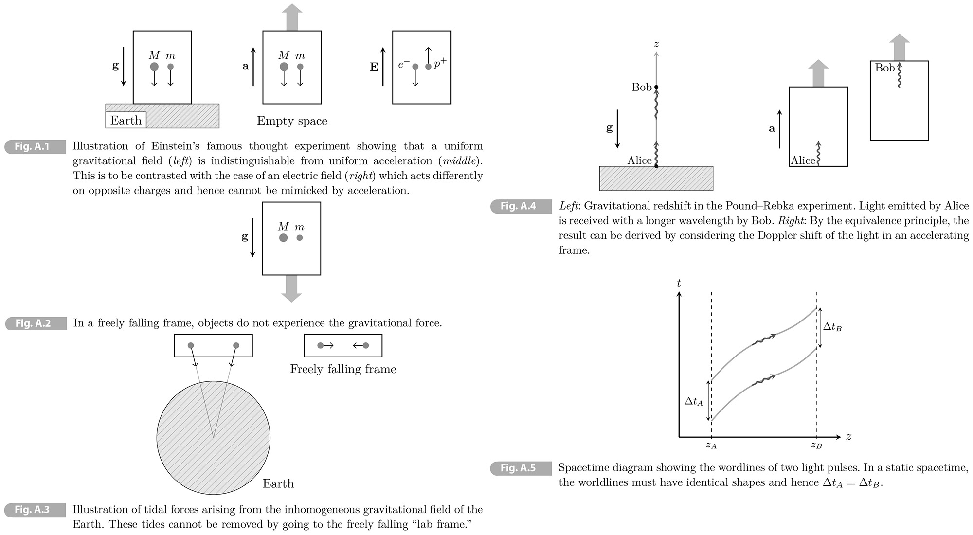
Imagine being confined to a sealed box. see (Fig. A.1) Consider first the case (right) where the box is sitting in an electric field. We can tell the situation easily by studying the motion of an electron and proton. However, in case of gravity, as Einstein's famous thought experiment, when we see two test particles with different masses are falling in exactly the same way, 𝐚 = -𝐠, we cannot tell the difference between a uniform gravitational field (left) and uniform acceleration (left). We conclude that
A uniform gravitational field is indistinguishable from uniform acceleration.
A corollary of this observation is the fact that the effects of gravity can be removed by falling freely, 𝐚 = 𝐠, the particles in the box will not fall to the ground. Einstein called this his "happiest thought": a freely falling observer doesn't feel a gravitational field (see Fig. A.2).
Einstein said that there is no experiment that distinguish uniform acceleration from a uniform gravitational field. This generalization of the WEP is called the Einstein equivalence principle (EEP).It implies that, in a small region (so that the gravitational field is approximately uniform), we can always find coordinates so that there is no acceleration. THese coordinates correspond to a local inertial frame where the spacetime is approximately Minkowsy space. Said differently:
In a small region, the laws of physics reduces to those of special relativity.
As we will see, the EEP suggests that the effects of gravity are associated with the curvature of spacetime which becomes relevant on larger scales where the field cannot be approximated as being uniform.
Consider a box that is freely falling towards the Earth (see Fig. A.3). We again drop two test particles. They will then accelerate toward each other because of a force towards the center of the Earth. This is an example of a tidal force arising from the non-uniformity of the gravitational field. Note that these tidal forces cause initially "parallel" trajectories to converge. As we will see, this violation of Euclidean geometry is a manifestation of the curvature of spacetime.
A.2.2 Gravity as Curved Spacetime
We will give a simple argument which will link the equivalence principle rather directly to the curvature of spacetime. For clarity, we will restore light speed 𝑐 factor in this section.
Let us begin by describing a famous observational consequence of the equivalence principle, the gravitational redshift. Consider Alice and Bob in a uniform gravitational field of strength 𝑔 in the negative 𝑧-direction (see Fig/ A.4. They are at heights 𝑧𝛢 = 0 and 𝑧𝛣 = 𝘩, respectively. If Alice send out a light signal with wavelength 𝜆𝛢 = 𝜆0. What is the wavelength 𝜆𝛣 received by Bob? By the equivalence principle, we can take Alice and Bob to be moving with acceleration 𝐚 = 𝐠 in the positive 𝑧-direction in Minkowski spacetime. (see Fig. A,4). Assuming ∆𝑣/𝑐 to be small, the light reaches Bob after a time ∆𝑡 ≈ 𝘩/𝑐. By this time Bob's velocity has increased by ∆𝑣 = 𝑔∆𝑡 = 𝑔 𝘩/𝑐. Due to the Doppler effect, the received light will have a silghtly longer wavelength, 𝜆𝛣 = 𝜆0 + ∆𝜆, with
(A.51) ∆𝜆/𝜆0 = ∆𝑣/𝑐 = 𝑔𝘩/𝑐2.
By the equivalence principle, light emitted from the ground with wavelength 𝜆0 must therefore be "redshifted" by the amount
(A.52) ∆𝜆/𝜆0 = ∆𝛷/𝑐2,
where ∆𝛷 = 𝑔𝘩 is the change in the gravitational potential. This gravitational redshift was first measured by Pound and Rebka in 1959.
We can also think of the gravitational redshift as an effect of time dilation. The period of the emitted light is 𝛵𝛢 = 𝜆𝛢/𝑐 and that of the received light is 𝛵𝛣 = 𝜆𝛣/𝑐. The resukt in (A.52) then implies that
(A.53) 𝛵𝛣 = [1 + (𝛷𝛣 - 𝛷𝛢)/𝑐2] 𝛵𝛢.
We conclude that time run slower in a region of stronger gravity (smaller 𝛷). In the example above, we have 𝛷𝛢 < 𝛷𝛣 (Alice feels a stronger gravitational field than Bob), so that 𝛵𝛢 < 𝛵𝛣 (time runs slower for Alice than for Bob). The result holds for any type of clock in a gravitational field. It also applies to the heart rate of the observer. This means that Alice will see Bob aging more rapidly. This "gravitational twin paradox" has been tested with atomic clocks on planes.3
Let us finally see why all of this implies that spacetime is curved. Anlie now sends out two pulses of light, eprataed by a time interval ∆𝑡𝛢 (as measured by her clock). Bob receives the signals spaced out by ∆𝑡𝛣 (as measured by his clock). Fig. A.5 shows the corresponding spacetime diagram. When in the diagram, drawing the congruent worldline ∆𝑡𝛣 = ∆𝑡𝛢, in apparent contradiction to (A.53), we implicitly assumed that the spacetime is flat. The resolution to the paradox is to accept that the spacetime is curved.
To see this more explicitly, consider a spacetime is not given by d𝑠2 = -d𝑡2 + d𝐱2, but by
(A.54) d𝑠2 = -[1 + 2𝛷(𝐱)/𝑐2] d𝑡2 + d𝐱2, with 𝛷 ≪ 𝑐2.
In these coordinates, the interval ∆𝑡 is the same for Alice and Bob, but their observed proper times are different. The proper time interval between the signals sent by Alice is
(A.55) ∆𝜏𝛢 = √[-𝑔00(𝐱)] ∆𝑡 = √[1 + 2𝛷𝛢/𝑐2] ∆𝑡 ≈ (1 + 𝛷𝛢/𝑐2) ∆𝑡,
where we used ∆𝐱 = 0 and expanded to first order in small 𝛷𝛢 = 𝛷(𝐱𝛢). similarly, the proper time between the signals received by Bob is
(A.56) ∆𝜏𝛣 = (1 + 𝛷𝛣/𝑐2) ∆𝑡.
Combining (A.55) and (A.56), we find
(A.57) ∆𝜏𝛣 = (1 + 𝛷𝛣/𝑐2) (1 + 𝛷𝛣/𝑐2)-1 ∆𝜏𝛢 ≈ [1 + (𝛷𝛣 - 𝛷𝛢)/𝑐2] ∆𝜏𝛢,
which is the same as (A.53). The time dilation has therefore been explained by the geometry of spacetime.
A.3 Motion in Curved Spacetime
General relativity contains two key ideas: (1) "spacetime curvature tells matter how to move" (equivalence principle) and (2) "matter tells spacetime how to curve" (Einstein equation). We will show that in the absence of any non-gravitational force, particles move along special paths in the curved space time called geodesics.
A.3.1 Relativistic Action
The action of a relativistic point particle is
(A.58) 𝑆 = -𝑚 ∫ d𝜏,
where 𝜏 is the proper time along the wordline of the particle and 𝑚 is its mass. The action must be a Lorentz scalar, so that all observers compute the same value for it. All observers will agree on the amount of time that elapsed on a clock carried by the moving particle.
As a useful consistency check, we evaluate the action (A.58) for a particular observer in Minkowski spacetime. Using (A.22), the action can be written as following integral over time
(A.59) 𝑆 = -𝑚 ∫ d𝑡 √(1 - 𝑣2), where 𝑣2 = 𝛿𝑖𝑗𝑥̇𝑖𝑥̇𝑗.
For 𝑣 ≪ 1, the integrand is -𝑚 + 1/2 𝑚𝑣2. We see that the Lagrangian is simply the kinetic energy of the particle plus a constant that doesn't affect the equation of motion.
Substituting the line element (A.54) into (A.58), we get
(A.60) 𝑆 = -𝑚 ∫ d𝑡 √[(1 + 2𝛷) - 𝑣2] ≈ ∫ d𝑡 ( -𝑚 + 1/2 𝑚𝑣2 - 𝑚𝛷 + ∙ ∙ ∙ ),
where we expanded the square root for small 𝑣 and 𝛷. We see that the metric perturbation 𝛷 indeed plays the role of the gravitational potential in Newtonian gravity. It is now also obvious why the inertial mas (appearing in the kinetic term 1/2 𝑚𝑣2) is the same as the gravitational mass (appearing in the potential 𝑚𝛷).
A.3.2 Geodesic Equation
Let us now use the action (A.58) to study the motion of particles in a general curved spacetime with metric 𝑔𝜇𝜈(𝑡, 𝐱). Consider an arbitrary timelike curve 𝓒 connecting two points 𝑝 and 𝑞 (see Fig. A.6). A geodesic is the preferred curve for which the action is an extremum. We first introduce a parameter 𝜆 to label points along the curve, 𝑥𝜇(𝜆), with 𝓒(0) = 𝑝 and 𝓒(1) = 𝑞. The action for curve 𝓒 can be written as
(A.61) 𝑆[𝑥𝜇(𝜆)] = -𝑚 ∫10 d𝜆 √(-𝑔𝜇𝜈 d𝑥𝜇/d𝜆 d𝑥𝜈/d𝜆).
This action has an extremum if path satisfies the geodesic equation
(A.62) d2𝑥𝜇/d𝜏2 + 𝛤𝜇𝛼𝛽 d𝑥𝛼/d𝜏 d𝑥𝛽/d𝜏 = 0,
where 𝜏 is the proper time along the curve and
(A.63) 𝛤𝜇𝛼𝛽 ≡ 1/2 𝑔𝜇𝜆(∂𝛼𝑔𝛽𝜆 + ∂𝛽𝑔𝛼𝜆 - ∂𝜆𝑔𝛼𝛽)
is the Christoffel symbol (or "connection coefficient").
Derivation Consider a small variation of path 𝑥𝜇 → 𝑥𝜇 + 𝛿𝑥𝜇. The corresponding variation of the action is
(A.64-5) 𝛿𝑆 ≡ 𝑆[𝑥𝜇 + 𝛿𝑥𝜇] - 𝑆[𝑥𝜇]
= 𝑚 ∫10 d𝜆 1/2𝐿 (𝛿𝑔𝜇𝜈 d𝑥𝜇/d𝜆 d𝑥𝜈/d𝜆 + 2𝑔𝜇𝜈 d𝑥𝜇/d𝜆 d𝛿𝑥𝜈/d𝜆), where 𝐿2 ≡ -𝑔𝜇𝜈 d𝑥𝜇/d𝜆 d𝑥𝜈/d𝜆 = (d𝜏/d𝜆)2.
Since d𝜏/d𝜆 = 𝐿, (A.64) becomes
(A.66) 𝛿𝑆 = 𝑚 ∫ d𝜏 (d𝜆/d𝜏) 1/2𝐿 [𝛿𝑔𝜇𝜈𝐿2ẋ𝜇ẋ𝜈 + 2𝐿2𝑔𝜇𝜈ẋ𝜇 𝛿(ẋ𝜈)] = 𝑚 ∫ d𝜏 (d𝜆/d𝜏) 1/2 [∂𝛼𝑔𝜇𝜈 𝛿𝑥𝛼ẋ𝜇ẋ𝜈 + 2𝑔𝜇𝜈𝑥̇𝜇 𝛿(ẋ𝜈)],
where ẋ𝜇 ≡ d𝑥𝜇/d𝜏. Integrating the second term of (A.66) by parts, we get
(A.67) 𝛿𝑆 = 𝑚 ∫ d𝜏 (1/2 ∂𝛼𝑔𝜇𝜈ẋ𝜇ẋ𝜈 𝛿𝑥𝛼 - 𝑔𝜇𝜈ẍ𝜇 𝛿𝑥𝜈 - ∂𝛼𝑔𝜇𝜈ẋ𝛼ẋ𝜇 𝛿𝑥𝜈)
In the last term, we can replace ∂𝛼𝑔𝜇𝜈 with 1/2 (∂𝛼𝑔𝜇𝜈 + ∂𝜇𝑔𝛼𝜈) because it is contracted with an object that is symmetric in 𝛼 and 𝜇. After relabeling of indices, we get
(A.68) 𝛿𝑆 = -𝑚 ∫ d𝜏 [𝑔𝜇𝜈ẍ𝜇 + 1/2 (∂𝛼𝑔𝛽𝜈 + ∂𝛽𝑔𝛼𝜈 - ∂𝜈𝑔𝛼𝛽) ẋ𝛼ẋ𝛽] 𝛿𝑥𝜈.
Factoring out the metric 𝑔𝜇𝜈, we can write this as
(A.69) 𝛿𝑆 = -𝑚 ∫ d𝜏 𝑔𝜇𝜈 (ẍ𝜇 + 𝛤𝜇𝛼𝛽 d𝑥𝛼/d𝜏 d𝑥𝛽/d𝜏) 𝛿𝑥𝜈, where 𝛤𝜇𝛼𝛽 is the Christoffel symbol in (A.63).
In order for 𝛿𝑆 to vanish for arbitrary 𝛿𝑥𝜈, the bracket in (A.69) must vanish and we obtain the geodesic equation (A.62). ▮
We see that the simple action (A.58) gives rise to a relatively complex geodesic equation, which is often applied in the cosmological context (see Section 2.2.1). It is also useful to the geodesic equation in terms of 4-velocity 𝑈𝜇 = d𝑥𝜇/d𝜏 Using the chain rule to write
(A.70) d/d𝜏 𝑈𝜇(𝑥𝛼(𝜏)) = d𝑥𝛼/d𝜏 ∂𝑈𝜇/∂𝑥𝛼 = 𝑈𝛼 ∂𝑈𝜇/∂𝑥𝛼,
equation (A.62) becomes
(A.71) 𝑈𝛼 (∂𝑈𝜇/∂𝑥𝛼 + 𝛤𝜇𝛼𝛽𝑈𝛽) = 0.
The term in the bracket is so-called covariant derivative of the 4-vector 𝑈𝜇 which we write as
(A.72) ∇𝛼𝑈𝜇 ≡ ∂𝛼𝑈𝜇 + 𝛤𝜇𝛼𝛽𝑈𝛽.
The geodesic equation can then be written in the following compact way:
(A.73) 𝑈𝛼∇𝛼𝑈𝜇 = 0.
We will see below this form of geodesic equation can also be derived directly by the concept "parallel transport" of the 4-velocity.
Newtonian limit
In Newtonian gravity, the equation of motion for a test particle in a gravitational field is
(A.74) d2𝑥𝑖/d𝑡2 = -∂𝑖𝛷.
Let us recover this result from the Newtonian limit of the geodesic equation (A.62). The Newtonian approximation assumes that (1) particles are moving slowly (relative to 𝑐), (2) the gravitational field is weak (so can be treated as a perturbation of Minkowski space), and (3) the field is also static. The first condition means that
(A.75) d𝑥𝑖/d𝜏 ≪ d𝑡/d𝜏,
so that (A.62) becomes
(A.76) d2𝑥𝜇/d𝜏2 + 𝛤𝜇00 (d𝑡/d𝜏)2 = 0.
In the static, weak limit, we write the metric (and its inverse) as
(A.77) 𝑔𝜇𝜈 = 𝜂𝜇𝜈 + 𝘩𝜇𝜈, 𝑔𝜇𝜈 = 𝜂𝜇𝜈 - 𝘩𝜇𝜈, [verification needed]
where the perturbation is small, ∣𝘩𝜇𝜈∣ ≪ 1, and time independent. The first order in 𝘩𝜇𝜈, the relevant component of Christoffel symbol is
(A.78) 𝛤𝜇00 = 1/2 𝑔𝜇𝜆(∂0𝑔𝜆0 + ∂0𝑔𝜆0 - ∂𝜆𝑔00) = -1/2 𝜂𝜇𝑗∂𝑗𝘩00.
The 𝜇 = 0 component of (A.76) reads d2𝑡/d𝜏2 = 0, so that d𝑡/d𝜏 is a constant, while the 𝜇 = 𝑖 component becomes
(A.79) d2𝑥𝑖/d𝜏2 = 1/2 (d𝑡/d𝜏)2∂𝑖𝘩00.
Dividing both sides by (d𝑡/d𝜏)2, we get
(A.80) d2𝑥𝑖/d𝑡2 = 1/2 ∂𝑖𝘩00.
which matches (A.74) if
(A.81) 𝘩00 = -2𝛷.
Note that this result is consistent with (A.54).
Massless particles
For massless particles, (A.61) doesn't hold, while the general form of the geodesic equation still holds
(A.82) d2𝑥𝜇/d𝜆2 + 𝛤𝜇𝛼𝛽 d𝑥𝛼/d𝜆 d𝑥𝛽/d𝜆 = 0,
but 𝜆 cannot be identified with proper time. Instead we choose 𝜆 such that 𝑃𝜇 = d𝑥𝜇/d𝜆, where 𝑃𝜇 is 4- momentum of the particle. The geodesic equation for a massless particle can be written as 𝑃𝛼∇𝛼𝑃𝜇 = 0, with 𝑃𝜇𝑃𝜇 = 0 (see Section 2.2.1). [RE Wikipedia Four-momentum]
3 Accounting for time dilation effects is also essential for the operation of the GPS (Global Positioning System) [1]. The satellites used in GPS are about 20 000 km above the Earth where the gravitational field is four times weaker than that on the ground. Because of time dilation the clocks on the satellites tick faster by about 45 𝜇s per day. Correcting for the relativistic time dilation due to the motion of the orbiting clocks (at about 14 000 km/hr), the net effect is 38 𝜇s per day. To achieve a positional accuracy of 15 m, time throughout the GPS system must be known to an accuracy of 50 ns (the time required for light to travel 15 m). |
|
|