|
김관석
|
2024-12-07 19:52:00, 조회수 : 187 |
- Download #1 : BC_7d.jpg (928.5 KB), Download : 1

7.6 A Glimpse at CMB Polarization*
Measurement of the CMB polarlization are at the forefront of observational cosmology. In this section an introduction to the physics of CMB polarization will be given. The goal is to provide an intuitive understanding of E/B decomposition of the polarization signal and to explain why B-modes are a unique signature of primordial tensor modes.
7.6.1 Polarization from Scattering
Consider the scattering of radiation by a free electron as illustrated in Fog. 7.25. Imagine that the angle between the incoming and outgoing rays is 90∘; e.g. let the incoming and outgoing rays be in the directions -𝐱̂ and +𝐳̂, respectively. Even if the incoming radiation is unpolarized, the outgoing radiation will become polarized, This is because the polarization direction must be transverse to the direction of propagation. For the scattering shown in the left panel of Fig. 7.25 all of the intensity along the 𝑧-axis blocked and only that along the 𝑦-axis is transmitted. The net result is polarization in the direction 𝐲̂.
In general, radiation will come from all directions and scatter into all directions. If the incident radiation is isotropic, then the net result after scattering will still be unpolaarized radiation. To see this, consider adding a ray of ulpolarized radiation in the direction -𝐲̂ as the right panel in Fig. 7.25. The sum of the polarized radiation created by the two incoming rays will be unpolarized radiation. To create a net polarization, we require anisotropy in the incoming radiation.
Exercise 7.5 Show with a sketch that the scattering of dipolar anisotropy also does not lead to a net polarization.
[Solution] If we make the modified Fig. 7.26 where the intensity of the radiation coming from ±𝐱̂ is the same as that coming from ±𝐲̂ and 𝐱̂ is for cold and hot region while 𝐲̂ is for dipolar anisotropy, it becomes a sketch that the scattering of dipolar anisotropy also does not lead to a net polarization. ▮
Fig. 7.26 shows that polarization is generated if the incident radiation has a quadrupolar anisotropy. The intensity of the radiation coming from the directions ±𝐲̂ is now larger than that coming from ±𝐱̂. Then the outgoing radiation will be polarized in the 𝐱̂-direction. It is useful to remember that the polarization direction of the outgoing radiation is aligned with the hot regions.
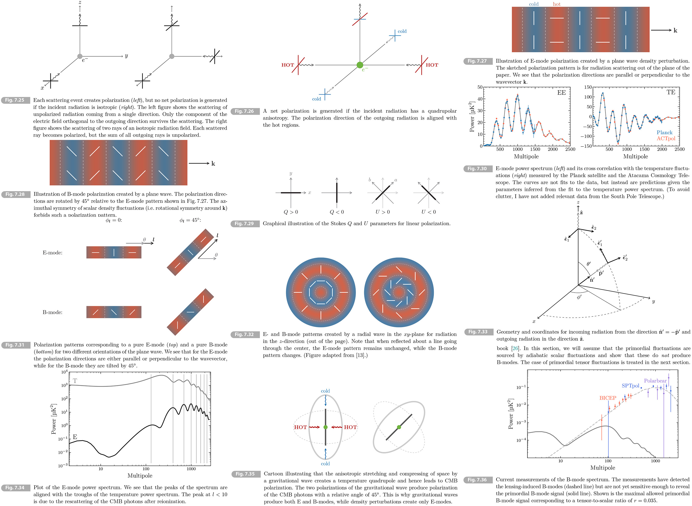
The polarization pattern observed on the sky will be the result of the scattering of the temperature inhomogeneities in the primordial plasma. These inhomogeneities are best described in a Fourier decomposition, with each mode describing a plain wave perturbation. It is useful to first determine the polarization generated by a single plane wave. Consider a plane wave photon density perturbation propagating in a direction transverse to the line-of-sight (see Fig. 7.27). The plane wave corresponds to hot and cold modulations of the photon temperature. Using our earlier assertion that the polarization is aligned with the hot regions, we predict the polarization pattern shown in Fig. 7.27. The polarization directions are ether parallel or perpendicular to the wavevector 𝐤. We call such a polarization pattern an E-mode.
Rotating all polarization directions by 45 degrees would give so-called B-mode polarization (see Fig. 7.28). By symmetry, this type of polarization pattern cannot be generated by scalar (density) fluctuations. The B-mode patterns is a key signature of gravitational waves in the early universe. We will discuss this in detail in Section 7.6.5.
7.6.2 Statistics of CMB Polarization
Stokes parameters
Consider a monochromatic electromagnetic plane wave propagating in the 𝑧-direction. The electric field of the wave is
(7.156) 𝑬(𝑧, 𝑡) = Re[(𝐸𝑥𝐱̂ + 𝐸𝑦𝐲̂) 𝑒𝑖(𝑘𝑧 - 𝜔𝑡)], [Re(𝑥): 'real part' of 𝑥]
where 𝜔 = 𝑘𝑐. We can define the complex amplitudes as 𝐸𝑥 = ∣𝐸𝑥∣𝑒𝑖𝜑𝑥 and 𝐸𝑦 = ∣𝐸𝑦∣𝑒𝑖𝜑𝑦. At a given location, taking 𝑧 = 0, we have
(7.157) 𝑬(𝑡) = ∣𝐸𝑥∣ cos(𝜔𝑡) 𝐱̂ + ∣𝐸𝑦∣ cos(𝜔𝑡 - 𝜑) 𝐲̂,
where we defined 𝜑 ≡ 𝜑𝑦 - 𝜑𝑥 and chose the origin of time so that 𝜑𝑥 ≡ 0. In general, the field vector in (7.157) traces out an ellipse in the 𝑥𝑦-plane. For 𝜑 = 0 (or π), the 𝑥- and 𝑦- components of the field oscillate in phase (anti-phase) and the ellipse degenerates into a line. We say that the wave is linearly polarized. For 𝜑 = ±π/2, the wave is circularly polarized.
The polarization of electromagnetic radiation is then defined by the Stokes parameters
(7.158) 𝐼 ≡ ∣𝐸𝑥∣2 + ∣𝐸𝑦∣2, 𝑄 ≡ ∣𝐸𝑥∣2 - ∣𝐸𝑦∣2, 𝑈 ≡ 2∣𝐸𝑥∣∣𝐸𝑦∣ cos(𝜑), 𝑉 ≡ 2∣𝐸𝑥∣∣𝐸𝑦∣ sin(𝜑),
where 𝐼 measures the intensity of the radiation, while 𝑄, 𝑈, 𝑉 describes its polarization state. The expression in (7.158) describes fully polarized radiation, with 𝐼2 = 𝑄2 + 𝑈2 + 𝑉2, which the CMB is certainly not; the polarization amplitude of the CMB is less than 10% of the temperature anisotropy. Recall that, in SI units, the energy density of an elevtromagnetic wave is 𝜌 = 𝜀0∣𝐸∣2 and its intensity is 𝓘 = 𝜌𝑐 = 𝑐𝜀0∣𝐸∣2. Averaged over many oscillation periods, we have
(7.159) ⟨𝓘⟩ = 𝑐𝜀0⟨∣𝐸∣2⟩ = 1/2 𝑐𝜀0(∣𝐸𝑥∣2 + ∣𝐸𝑦∣2) = 1/2 𝑐𝜀0𝐼.
In units with 𝑐 = 𝜀0 ≡ 1, we get 𝐼 = 2⟨𝓘⟩, so that the Stokes parameter 𝐼 indeed is a measure of the time-averaged intensity.
The Stokes parameter 𝑉 vanishes for linear polarization (with 𝜑 = 0, π). Since circular polarization usually isn't produced in the early universe, we will set 𝑉 ≡ 0 in the following. Then 𝑄 and 𝑈 describe the linear polarization of the radiation. 𝑄 is the difference between the intensity of the radiation along 𝑥-axis, ∣𝐸𝑥∣2 and that along 𝑦-axis, ∣𝐸𝑦∣2. Radiation polarized along 𝑥-axis has 𝑄 > 0, while Radiation polarized along 𝑦-axis has 𝑄 < 0. Similarly, the parameter 𝑈 can be thought of as the difference in the intensity along two contribute axes 𝑎 and 𝑏 that are rotated counterclockwise by 45∘ (see Fig. 7.20):
(7.160) 𝑈 = ∣𝐸𝑎∣2 - ∣𝐸𝑏∣2 = 2Re[𝐸𝑥𝐸𝑦*],
where we used that 𝐸𝑥,𝑦 = (𝐸𝑎 ± 𝑖𝐸𝑏)/√2. Radiation polarized along the 𝑎-axis has 𝑈 > 0, while radiation polarized along 𝑏-axis has 𝑈 < 0.
Rotating the 𝑥 and 𝑦 axes counterclockwise by an angle 𝜙 transforms the Stokes parameters
(7.161) ⌈𝐸𝑥ʹ⌉ = ⌈ cos(𝜙) sin(𝜙)⌉ ⌈𝐸𝑥⌉ * IPAD view (7.161) ⌈𝐸𝑥ʹ⌉ = ⌈ cos(𝜙) sin(𝜙)⌉ ⌈𝐸𝑥⌉ * PC view
⌊𝐸𝑦ʹ⌋ ⌊-sin(𝜙) cos(𝜙)⌋ ⌊𝐸𝑦⌋, ⌊𝐸𝑦ʹ⌋ ⌊-sin(𝜙) cos(𝜙)⌋ ⌊𝐸𝑦⌋,
⌈𝑄ʹ⌉ = ⌈ cos(2𝜙) sin(2𝜙)⌉ ⌈𝑄⌉ ⌈𝑄ʹ⌉ = ⌈ cos(2𝜙) sin(2𝜙)⌉ ⌈𝑄⌉
⌊𝑈ʹ⌋ ⌊-sin(2𝜙) cos(2𝜙)⌋ ⌊𝑈⌋. ⌊𝑈ʹ⌋ ⌊-sin(2𝜙) cos(2𝜙)⌋ ⌊𝑈⌋.
The transformation of the Stokes parameters can also be written as
(7.162) 𝑄ʹ ± 𝑖𝑈ʹ = 𝑒∓2𝑖𝜙(𝑄 ± 𝑖𝑈),
which shows that polarization transform like a spin-2 field. [RE Wikipedia Spin (physics)] To avoid this ambiguity, we will introduce the coordinate-independent E- and B-modes of the polarization field.
Decomposition into E- and B-modes
On scales smaller than a few degrees the sky cam be approximated as flat. This flat-sky limit greatly simplifies the mathematical treatment of CMB polarization, so we will use the following. Let 𝜽 = (𝜃𝑥, 𝜃𝑦) be the position on a flat region of the sky and definethe symmetric and trace-free polarization tensor as
(7.163) 𝑃𝑎𝑏(𝜽) ≡ ⌈𝑄(𝜽) 𝑈(𝜽)⌉ * IPAD view (7.163) 𝑃𝑎𝑏(𝜽) ≡ ⌈𝑄(𝜽) 𝑈(𝜽)⌉ * PC view
⌊𝑈(𝜽) -𝑄(𝜽)⌋ ⌊𝑈(𝜽) -𝑄(𝜽)⌋
Being made out of the Stokes parameters, this polarization tensor also transforms under a rotation of the coordinate. However by taking spatial derivatives of 𝑃𝑎𝑏 we can define two quantities invariant under rotations
(7.164) ∇2𝐸 ≡ ∂𝑎∂𝑏𝑃𝑎𝑏, ∇2𝛣 ≡ 𝜖𝑎𝑐∂𝑏∂𝑐𝑃𝑎𝑏,
where 𝜖𝑎𝑐 is the antisymmetric tensor. In fact, these definitions of E- and B-modes even hold beyond the flat-sky limit if we promote the derivatives to covariant derivatives on the sphere. Writing (7.164) out in terms of the Stokes parameters, we get
(7.165) ∇2𝐸 ≡ (∂𝑥2 - ∂𝑦2)𝑄 + 2∂𝑥∂𝑦𝑈, ∇2𝛣 ≡ (∂𝑥2 - ∂𝑦2)𝑈 - 2∂𝑥∂𝑦𝑄.
We note that the relation between the E- and B-modes and the Stokes parameters is non-local.
The E/B decomposition of the polarization is similar to the decomposition of a vector field into a gradient of a scalar function and the curl of a vector
(7.166) 𝐕 = 𝛁𝐺 - 𝛁 × 𝐂,
where 𝛁 ⋅ 𝐂 = 0. Taking the divergence and the curl of the vector, we can isolate the two components
(7.167) ∇2𝐺 = 𝛁 ⋅ 𝐕, ∇2𝐂 = 𝛁 × 𝐕,
which indeed looks very similar to (7.164). This decomposition of a vector field into a curl-free gradient part and a divergence-free curl part also explains the names E-mode and B-mode: in electrostatics, the electric field has vanishing curl, 𝛁 × 𝐄 = 0, [RE 𝛁 × 𝐄 = -∂𝐁/∂𝑡 in Maxwell's equation] while a magnetic field has zero divergence, 𝛁 ⋅ 𝐁 = 0.
Polarization power spectra
The CMB map is now described by the temperature 𝛵 and the polarization modes 𝐸 and 𝛣, which collectively call 𝑋 ≡ {𝛵, 𝐸, 𝛣}. The main benefit of working in the flat-sky limit is that we can use ordinary Fourier transform instead of spherical harmonics
(7.168) 𝑋(𝒍) = ∫ d2𝜽 𝑋(𝜽) 𝑒-𝑖𝒍⋅𝜽,
where 𝒍 is the 2-dimensional wavevector conjugate to the position 𝜽. The relations in (7.165) imply that the Fourier components of the E- and B-modes satisfy
(7.169) 𝐸(𝒍) = [(𝑙𝑥2 - 𝑙𝑦2)𝑄(𝒍) + 2𝑙𝑥𝑙𝑦𝑈(𝒍)]/(𝑙𝑥2 + 𝑙𝑦2), 𝛣(𝒍) = [(𝑙𝑥2 - 𝑙𝑦2)𝑈(𝒍) - 2𝑙𝑥𝑙𝑦𝑄(𝒍)]/(𝑙𝑥2 + 𝑙𝑦2).
We should confirm that although 𝑄(𝒍) and 𝑈(𝒍) transform under a rotation of the 𝜽𝑥- and 𝜽𝑦-axes, 𝐸(𝒍) and 𝛣(𝒍) are invariant. The power spectra of the fluctuations are defined as
(7.170) ⟨𝑋(𝒍)𝑌(𝒍ʹ)⟩ = (2π)2𝛿𝐷(𝒍 + 𝒍ʹ)𝐶𝑙𝑋𝑌,
where 𝑋, 𝑌 = {𝛵, 𝐸, 𝛣}. In principle, this corresponds to six different spectra. But in practice only fiur spectra of them are expected to be nonzero. To see this, consider a reflection about 𝑥-axis (called a parity inversion).
(7.171) 𝜃𝑦 → -𝜃𝑦, 𝑄 → 𝑄, 𝑈 → -𝑈, 𝑙𝑥 → 𝑙𝑥, 𝑙𝑦 → -𝑙𝑦.
From (7.169) we see that E-mode is invariant under this reflection, while the B-mode change sign:
(7.172) 𝐸(𝒍) → 𝐸(𝒍), 𝛣(𝒍) → -𝛣(𝒍).
The field 𝐸 is therefore a parity-even scalar field (like 𝛵), while 𝛣 is a parity-odd pseudoscalar field. IF the physics of the primordial universe is parity conserving, then we expect 𝐶𝑙TB = 𝐶𝑙EB = 0.
On the full sky, we have to use spherical harmonics to describe the polarization field and generalize our definitions of E- and B-modes. We will just sketch the logic and leave the complicate mathematical details to [20. 21].
We saw that polarization is a spin-2 field, cf. (7.162). So we can't use ordinary scalar spherical harmonics to describe its decomposition into multipole moments. Instead we must use so-called spin-weighted sperical harmonics [20, 21]. Then the polarization field can be written as
(7.173) 𝑄(𝐧̂) ± 𝑖𝑈(𝐧̂) = ∑𝑙𝑚 𝑎±2,𝑙𝑚 ±𝑌𝑙𝑚(𝐧̂),
where the explicit forms of the spin-2 spherical harmonics ±𝑌𝑙𝑚(𝐧̂) can be found in [20, 21]. The multipole coefficient 𝑎2,𝑙𝑚 and 𝑎-2,𝑙𝑚 can be combined into parity even and parity-odd combinations:
(7.174) 𝑎𝑙𝑚𝐸 ≡ -(𝑎2,𝑙𝑚 + 𝑎-2,𝑙𝑚)/2, 𝑎𝑙𝑚𝛣 ≡ -(𝑎2,𝑙𝑚 + 𝑎-2,𝑙𝑚)/2𝑖,
which are multipole coefficients of the E- and B-modes:
(7.175) 𝐸(𝐧̂) = ∑𝑙𝑚 𝑎𝐸,𝑙𝑚 𝑌𝑙𝑚(𝐧̂), 𝛣(𝐧̂) = ∑𝑙𝑚 𝑎𝛣,𝑙𝑚 𝑌𝑙𝑚(𝐧̂).
The polarization power spectra are then defined in the usual way:
(7.176) ⟨𝑎𝑙𝑚𝑎𝑙ʹ𝑚ʹ𝐸*⟩ = 𝐶𝑙TE𝛿𝑙𝑙ʹ𝛿𝑚𝑚ʹ, ⟨𝑎𝑙𝑚𝐸𝑎𝑙ʹ𝑚ʹ𝐸*⟩ = 𝐶𝑙EE𝛿𝑙𝑙ʹ𝛿𝑚𝑚ʹ, ⟨𝑎𝑙𝑚𝛣𝑎𝑙ʹ𝑚ʹ𝛣*⟩ = 𝐶𝑙BB𝛿𝑙𝑙ʹ𝛿𝑚𝑚ʹ.
CMB polarization was first detected in 2002 by the Degree Angular Scale Interferomer (DASI) [22]. It has sice been measured with increasing precision by the WMAP and Planck satellites, as well as a number of ground-based experiments, Fig. 7.30 shows the TE and EE spectra measured by Planck [2] and ACT [23].
7.6.3 Visualizing E- and B-modes
We will relate the formal definitions of E- and B-modes to the pictures in Section 7.6.1. Wee return to the flat-sky approximation. For simplicity we align the 𝑥-axis of our coordinates with the position vector 𝜽, and let 𝜙𝒍 be the angle of the wavevector 𝒍 = 𝑙[cos(𝜙𝒍), sin(𝜙𝒍)]. The Fourier modes in (7.169) then are
(7.177) 𝐸(𝒍) = +𝑄(𝒍) cos(2𝜙𝒍) + 𝑈(𝒍) sin(2𝜙𝒍), 𝛣(𝒍) = -𝑄(𝒍) sin(2𝜙𝒍) + 𝑈(𝒍) cos(2𝜙𝒍).
Inverting these expressions leads to write the Stokes parameters in terms of 𝐸 and 𝛣:
(7.178) 𝑄(𝒍) = 𝐸(𝒍) cos(2𝜙𝒍) - 𝛣(𝒍) sin(2𝜙𝒍), 𝑈(𝒍) = 𝐸(𝒍) sin(2𝜙𝒍) - 𝛣(𝒍) cos(2𝜙𝒍),
The polarization generated by a single plane wave then is
(7.179) 𝑄(𝜽) = Re[𝐸(𝒍) cos(2𝜙𝒍) - 𝛣(𝒍) sin(2𝜙𝒍) 𝑒𝑖𝒍⋅𝜽], 𝑈(𝜽) = Re[𝐸(𝒍) cos(2𝜙𝒍) + 𝛣(𝒍) sin(2𝜙𝒍) 𝑒𝑖𝒍⋅𝜽],
where the factor of 𝑒𝑖𝒍⋅𝜽 describes the modulation of the polarization amplitude induced by the plane wave perturbation. From this expression we can infer the polarization patterns corresponding to pure E- and B-mode created by a plane wave perturbation.
For a pure E-mode, we have
(7.180) 𝑄(𝜽) = Re[𝐸(𝒍) cos(2𝜙𝒍) 𝑒𝑖𝒍⋅𝜽], 𝑈(𝜽) = Re[𝐸(𝒍) sin(2𝜙𝒍) 𝑒𝑖𝒍⋅𝜽].
In the top of Fig. 7.31 The corresponding polarization pattern for two representative orientations of the wavevector 𝒍 was showed. In both cases, the polarization directions are parallel or perpendicular to the wavevector. This defining feature of E-mode polarization holds for its any orientation. Another way diagnose the presence of the E-mode is to rotate the coordinate system so that the 𝑥ʹ-axis is aligned with direction 𝒍. The Stokes 𝑈 parameter will then vanish and the polarization will be pure 𝑄. This is another coordinate-independent way define the E-mode.
For a pure B-mode, we have
(7.181) 𝑄(𝜽) = -Re[𝛣(𝒍) sin(2𝜙𝒍) 𝑒𝑖𝒍⋅𝜽], 𝑈(𝜽) = +Re[𝛣(𝒍) cos(2𝜙𝒍) 𝑒𝑖𝒍⋅𝜽].
In the bottom of Fig. 7.31, as before the corresponding polarization pattern for the same two representative orientations of the wavevector 𝒍 was showed. The polarization directions are now tilted by 45∘ with the respect to the wavevector, which is the defining characteristic of B-mode polarization. Rotating the coordinates so that the 𝑥ʹ-axis is aligned with direction 𝒍. The Stokes 𝑄 parameter would vanish and the polarization is pure 𝑈.
More complex polarization patterns arise from the superposition of the polarization patterns created by plane wave perturbations. In Fig. 7.32 we consider the polarization generated by a radial wave in the 𝑥𝑦-plane. The wave can be thought of as a superposition of plane waves with equal phases and amplitude, but different azimuthal angle 𝜙𝒍. We can convince ourselves that a superposition of the polarization patterns shown in Fig. 7.31 (for varying 𝜙𝒍) produces the polarization in Fig. 7.32. We see that the E-mode pattern alternates between being radial and tangential, while the B-mode polarization has a characteristic "swirl" pattern.
7.6.4 E-modes from Scalars
We will now discuss the contents with more equations and a larger degree of generality and follow the excellent treatment in Dodelson's book [Dodelson]. In this section we will assume that the primordial fluctuations are sourced by adiabatic scalar fluctuations and show that these do not produce B-modes.
Thomson scattering revisited
In Section 7.6.1 we saw graphically how unpolarized radiation becomes polarized by scattering. Mathematically this is described by the dependence of the scattering cross section on the polarization of incoming and the outgoing radiation. If the polarization direction of the incoming radiation is 𝛜̂ʹ and that of the outgoing radiation is 𝛜̂, then the differential cross section is
(7.182) d𝜎/d𝛺 = 3𝜎𝛵/8π ∣𝛜̂ ⋅ 𝛜̂ʹ∣2.
The dependence on 𝛜̂ ⋅ 𝛜̂ʹ enforces that only the component of the incoming polarization that is orthogonal to the direction of the outgoing radiation is transmitted.
Without loss of generality, we can take the direction of the outgoing radiation to be 𝐳̂ and 𝛜̂1 ≡ 𝐱̂ and 𝛜̂2 ≡ 𝐲̂ to be an orthogonal basis of polarizational vectots (see Fig. 7.33). The 𝑄-type polarization of the outgoing radiation is
(7.183) 𝑄(𝐳̂) = 𝛢 ∫ d𝛺ʹ 𝑓(𝐧̂ʹ) ∑2𝑗=1 (∣𝐱̂ ⋅ 𝛜̂ʹ𝑗∣2 - ∣𝐲̂ ⋅ 𝛜̂ʹ𝑗∣2),
where 𝑓(𝐧̂ʹ) is the distribution function of the incoming radiation and 𝛢 is the overall normalization (which would be fixed by the intensity of the incoming radiation). We assumed that incident radiation is unpolarized, so 𝑓(𝐧̂ʹ) doesn't depend on 𝛜̂ʹ𝑗. To evaluate the inner product in (7.183), we write the polarization basis of the incoming radiation in Cartesian coordinates
(7.184) 𝛜̂ʹ1 ≡ -𝜽̂ʹ = [-cos(𝜃ʹ) cos(𝜙ʹ), -cos(𝜃ʹ) sin(𝜙ʹ), sin(𝜃ʹ)], 𝛜̂ʹ2 ≡ -𝝓̂ʹ = [-sin(𝜙ʹ), cos(𝜙ʹ), 0]
We then get [using WolframAlpha]
(7.185) 𝑄(𝐳̂) = 𝛢 ∫ d𝛺ʹ 𝑓(𝐧̂ʹ) [cos2(𝜃ʹ) cos2(𝜙ʹ) + sin2(𝜙ʹ) - cos2(𝜃ʹ) sin2(𝜙ʹ) - cos2(𝜙ʹ)] = -𝛢 ∫ d𝛺ʹ 𝑓(𝐧̂ʹ) sin2(𝜃ʹ) cos(2𝜙ʹ)
The combination of angles in this integral is proportional to a sum of 𝑙 = 2 spherical harmonics, sin2(𝜃ʹ) cos(2𝜙ʹ) ∝[𝑌22 + 𝑌2,-2](𝐧̂ʹ); see (D.6) in Appendix D. By orthogonality of the spherical harmonics, the integral will pick out the 𝑙 = 2, 𝑚 = ±2 components of 𝑓(𝐧̂ʹ). We derived the crucial result that a nonzero 𝑄 will only be produced if the incident radiation has a nonzero quadrupole moment. We saw this in pictures before, but it is nice to have it drop out of the equations.
The 𝑈-type polarization of the outgoing radiation is defined with respect to the polarization basis 𝛜̂𝑎 = (𝐱̂ + 𝐲̂)/√2 and 𝛜̂𝑏 = (𝐱̂ - 𝐲̂)/√2, We then find [also using WolframAlpha]
(7.186) 𝑈(𝐳̂) = 𝛢 ∫ d𝛺ʹ 𝑓(𝐧̂ʹ) ∑2𝑗=1 [∣(𝐱̂ + 𝐲̂) ⋅ 𝛜̂ʹ𝑗∣2 - ∣(𝐱̂ - 𝐲̂) ⋅ 𝛜̂ʹ𝑗∣2] = -𝛢 ∫ d𝛺ʹ 𝑓(𝐧̂ʹ) sin2(𝜃ʹ) sin(2𝜙ʹ)
where we substituted (7.184) to obtain the result in the second line. The angular dependence of the integrand is now proportional to the difference of 𝑙 = 2 spherical harmonics, sin2(𝜃ʹ) sin(2𝜙ʹ) ∝ [𝑌22 - 𝑌2,-2](𝐧̂ʹ), so that again only the quadruople moment of 𝑓(𝐧̂ʹ) produces polarization.
Polarization from a single plane wave
WE would like to predict the polarization signals generated by the scattering of an inhomogeneous distributions of photons. We first write the perturbed photon distribution function as
(7.187) 𝑓(𝐧̂ʹ, 𝐱) = exp(𝐸/𝛵̄[1 + 𝛩(𝐧̂ʹ, 𝐱)] -1)-1 ≈ 𝑓̄ - d𝑓̄/(d ln 𝐸) 𝛩(𝐧̂ʹ, 𝐱)
It's convenient to describe the spatial dependence of the fluctuation s in Fourier space, 𝜭(𝐧̂ʹ, 𝐱) → 𝜭(𝐧̂ʹ, 𝐱). The fluctuations created by scalar density perturbations have an axial symmetry. The perturbations in the direction 𝐧̂ʹ only depend on magnitude of the wavevector 𝑘 and the angle defined by 𝜇ʹ = 𝐤̂ ⋅ 𝐧̂ʹ. We then write the temperature perturbation as an expansion in Legendre polynomials
(7.188) 𝛩(𝑘, 𝜇ʹ) = ∑𝑙 𝑖𝑙(2𝑙 + 1) 𝛩𝑙(𝑘) 𝑃𝑙(𝜇ʹ).
Only the 𝑙 = 2 quadrupole moment of this expansion leads to polarization. Substituting this quadrupole into (7.185) and (7.186), we get
(7.189) 𝑄(𝐳̂) ∝𝛩2(𝑘) ∫π0 d𝜃ʹ sin(𝜃ʹ) ∫2π0 d𝜙ʹ 𝛲2(𝜇ʹ) sin2(𝜃ʹ) cos(2𝜙ʹ), 𝑈(𝐳̂) ∝𝛩2(𝑘) ∫π0 d𝜃ʹ sin(𝜃ʹ) ∫2π0 d𝜙ʹ 𝛲2(𝜇ʹ) sin2(𝜃ʹ) sin(2𝜙ʹ).
To evaluate the angular integrals, we must first write 𝜇ʹ in terms of 𝜃ʹ and 𝜙ʹ. Following Dodelson [Dodelson], we will do this in three steps:
1. First, we take the wavevector to be parallel to 𝑥-axis, 𝐤∥𝐱̂. This gives
(7.190) 𝜇ʹ = 𝐤 ⋅ 𝐧̂ʹ = 𝐱̂ ⋅ 𝐧̂ʹ = 𝑛̂𝑥ʹ = sin(𝜃ʹ) cos(𝜙ʹ),
and hence [RE Appendix D.3 (D.13): 𝑃̄2 = 1/2 (3𝜇2 - 1)]
(7.191) 𝑃̄2(𝜇ʹ) = 3/2(𝜇ʹ)2 - 1/2 = 3/2[sin(𝜃ʹ) cos(𝜙ʹ)]2 - 1/2.
Only the first term of the Legendre polynomial survives the angular integration in (7.180) and we get
(7.192) 𝑄(𝐳̂, 𝐤∥𝐱̂) ∝ 4π/5 𝛩2(𝑘), 𝑈(𝐳̂, 𝐤∥𝐱̂) ∝0.
This is consistent with what we found before: the polarization created by density perturbations has vanishing Stokes parameter 𝑈 when the 𝑥-axis is aligned with the wavevector of the plane wave.
2. Next, we take the wavevector to lie in the 𝑥𝑦-plane, 𝐤⊥𝐲̂. Writing
(7.193) 𝐤̂ = [sin(𝜃𝑘), 0, cos(𝜃𝑘)].
we get
(7.194) 𝜇ʹ = 𝐤 ⋅ 𝐧̂ʹ = sin(𝜃𝑘) 𝑛̂𝑥ʹ + cos(𝜃𝑘) 𝑛̂𝑥ʹ = sin(𝜃𝑘) sin(𝜃ʹ) cos(𝜙ʹ) + cos(𝜃𝑘) cos(𝜃ʹ),
and hence
(7.195) 𝑃̄2(𝜇ʹ) = 3/2[sin(𝜃ʹ) cos(𝜙ʹ)]2 + ⋅ ⋅ ⋅ ,
where the ellipse stand for terms that lead to vanishing contributions when integrated against cos(2𝜙ʹ) or sin(2𝜙ʹ). The only difference with the relevant term in (7.191) is the extra factor of sin2(𝜃𝑘). WE therefore get
(7.196) 𝑄(𝐳̂, 𝐤⊥𝐱̂) ∝4π/5 𝛩2(𝑘), 𝑈(𝐳̂, 𝐤⊥𝐱̂) ∝0.
Projected onto the 𝑥𝑦-plane the direction of the wavevector is still aligned with the 𝑥-axis, so the Stokes parameter 𝑈 still vanishes.
3. Finally, we consider a wavevector pointing in an arbitrary direction. Its components are
(7.197) 𝐤̂ = [sin(𝜃𝑘) cos(𝜙𝑘), sin(𝜃𝑘) sin(𝜙𝑘), cos(𝜃𝑘)].
(7.198) 𝑄(𝐳̂, 𝐤) ∝ 4π/5 sin2(𝜃𝑘) cos(2𝜙𝑘) 𝛩2(𝑘), 𝑈(𝐳̂, 𝐤) ∝ 4π/5 sin2(𝜃𝑘) sin(2𝜙𝑘) 𝛩2(𝑘).
Comparison with (7.178) reveals that this is indeed a pure 𝐸-mode:
(7.199) 𝐸(𝐳̂, 𝐤) ∝ 4π/5 sin2(𝜃𝑘) 𝛩2(𝑘). 𝐸(𝐳̂, 𝐤) ∝ 0,
where we have implicitly used that 𝒍 is the projection of 𝐤 onto the plane of the sky to identify 𝜙𝑘 with 𝜙𝒍.
Exercise 7.6 Derive the result in (7.198)
[Solution] For a fluctuationh general wavevector 𝐤, using
(a) 𝐤̂ = [sin(𝜃𝑘) cos(𝜙𝑘), sin(𝜃𝑘) sin(𝜙𝑘), cos(𝜃𝑘)], 𝐧̂ = [sin(𝜃ʹ) cos(𝜙ʹ), sin(𝜃ʹ) sin(𝜙ʹ), cos(𝜃ʹ)].
(b) 𝜇ʹ ≡ 𝐤̂ ⋅ 𝐧̂ = sin(𝜃𝑘) cos(𝜙𝑘 sin(𝜃ʹ) cos(𝜙ʹ) + sin(𝜃𝑘) sin(𝜙𝑘 sin(𝜃ʹ) sin(𝜙ʹ) + cos(𝜃𝑘) cos(𝜃ʹ).
(c) 𝑃̄2(𝜇ʹ) = 3/2(𝜇ʹ)2 - 1/2 = 3/2 (sin2(𝜃𝑘) cos2(𝜙𝑘) [sin(𝜃ʹ) cos(𝜙ʹ)]2
+ sin2(𝜃𝑘) sin2(𝜙𝑘) [sin(𝜃ʹ) sin(𝜙ʹ)]2 + 2 sin2(𝜃𝑘) cos(𝜙𝑘) sin(𝜙𝑘) sin2(𝜃ʹ) cos(𝜙ʹ) sin(𝜙ʹ)) + ⋅ ⋅ ⋅ ,
Substituting this into (7.189), we get
(d) 𝑄(𝐳̂, 𝐤) ∝ 𝛩2(𝑘) ∫π0 d𝜃ʹ sin(𝜃ʹ) ∫2π0 d𝜙ʹ 𝛲2(𝜇ʹ) sin2(𝜃ʹ) cos(2𝜙ʹ)
∝ 4π/5 𝛩2(𝑘) sin2(𝜃𝑘) [cos2(𝜙𝑘) - sin2(𝜙𝑘)] = 4π/5 sin2(𝜃𝑘) cos(2𝜙𝑘) 𝛩2(𝑘).
(e) 𝑈(𝐳̂, 𝐤) ∝ 𝛩2(𝑘) ∫π0 d𝜃ʹ sin(𝜃ʹ) ∫2π0 d𝜙ʹ 𝛲2(𝜇ʹ) sin2(𝜃ʹ) sin(2𝜙ʹ)
∝ 4π/5 𝛩2(𝑘) sin2(𝜃𝑘) × 2 sin(𝜃𝑘) cos(𝜙𝑘) = 4π/5 sin2(𝜃𝑘) sin(2𝜙𝑘) 𝛩2(𝑘). ▮
Ultimately we need the result for a general line-of-sight 𝐧̂. To obtain this we perform 𝐳̂ → -𝐧̂ and 𝐧̂ = -𝐩. Since the E-mode is invariant under this rotation, we must simply replace cos(𝜃𝑘) with -𝐧̂ ⋅ 𝐤̂ and (7.199) becomes
(7.200) 𝐸(𝐧̂, 𝐤̂) ∝ 4π/5 [1 - (𝐧̂ ⋅ 𝐤̂)2] 𝛩2(𝑘), 𝛣(𝐧̂, 𝐤̂) ∝ 0.
This result assumes the flat-sky approximation and hence only applies to directions 𝐧̂ near the 𝑧-axis. The general result is much more complicated, but the same conclusion holds: no B-modes are generated by scalar density fluctuations.
Quadruple from velocity gradients
We saw that polarization is generated by the scattering of a quadrupolar anisotropy. But in the tight-coupling regim, this anosotropy is erased by the frequent scattering of the photons. Polarization is therefore only generated near recombination when anisotropies grow by free streaming. Since the electron density drops sharply at recombination there is only a short time window of the significant polarization of the CMB.
In density perturbations the quadrupole moment is produced by velocity gradients in the photon-baryon fluid. Refer to Appendix B for the explicit derivation using Boltzmann equation. Here a more heuristic explanation will be given [27]. Consider scattering at 𝐱0. The scattered photon came from a position 𝐱 = 𝐱0 + 𝓁𝛾𝐧̂ʹ, where 𝓁𝛾 = 𝛤-1 is the mean free path. The velocity of photon of the photon-baryon fluid at that position was
(7.201) 𝐯𝑏(𝐱) ≈ 𝐯𝑏(𝐱0) + 𝓁𝛾𝐧̂ʹ ⋅ 𝛁 𝐯𝑏(𝐱0).
The temperature seen by the scatterer at 𝐱0 is Doppler shifted and hence given by
(7.202) 𝛩(𝐱0, 𝐧̂ʹ) ≡ 𝛿𝛵(𝐱0, 𝐧̂ʹ)/𝛵̄ = 𝐧̂ʹ ⋅ [𝐯𝑏(𝐱) - 𝐯𝑏(𝐱0)] ≈ 𝓁𝛾𝑛̂𝑖ʹ𝑛̂𝑗ʹ∂𝑖(𝐯𝑏)𝑗.
Being quadradtic in 𝐧̂ʹ, the induced temperature anisotropy has the required quadrupole component 𝛩2. The Fourier transform of (7.202) is
(7.203) 𝛩(𝐤, 𝐧̂ʹ) = ∫ d3 𝑥 𝑒-𝑖𝐤, 𝐱 𝛩(𝐱, 𝐧̂ʹ) = 𝓁𝛾𝑛̂𝑖ʹ𝑛̂𝑗(𝑖𝑘𝑖)(𝑗𝑘𝑗 𝑣𝑏) = -𝑘/𝛤 𝑣𝑏 (𝐤̂ ⋅ 𝐧̂ʹ)2 ⊂ -2/3 𝑘/𝛤 𝑣𝑏 𝑃̄2(𝜇ʹ), [verification needed]
from which we can read off 𝛩2(𝑘).
E-mode spectrum
Let 𝐱0 now be a point on the surface of last-scattering. Using (7.200) and (7.203), the E-mode polarization created by a plane wave perturbation is
(7.204) 𝐸(𝐧̂, 𝐤) ∝ [1 - (𝐧̂ ⋅ 𝐤̂)2] 𝛩2(𝑘) 𝑒𝑖𝐤 ⋅ 𝐱0 ∝ 𝑘/𝛤 𝑣𝑏(𝜂*, 𝐤)(1 - 𝜇2) 𝑒𝑖𝑘𝜂0𝜇,
where we include the factor of 𝑒𝑖𝐤 ⋅ 𝐱0 to describe the modulation of the amplitude as a function of the position 𝐱0 = (𝜂0 - 𝜂*)𝐧̂ ≈ 𝜂0𝐧̂. Next we expand the exponential in spherical Bessel functions and extract the multipole moment 𝐸𝑙(𝐤). The details are given in Appendix B, where we find that
(7.205) 𝐸𝑙(𝐤) ∝ 𝑘/𝛤 𝑣𝑏(𝜂*, 𝐤) √(1 + 2)𝑙!/(1 - 2)𝑙! 𝑗𝑙(𝑘𝜂0)/(𝑘𝜂0)2.
For large 𝑙, the square root becomes 𝑙2 and the polarization transfer function is
(7.206) 𝛩𝐸,𝑙(𝑘) ≡ 𝐸𝑙(𝐤)/𝓡𝑖(𝐤) ∝ 𝑘/𝛤 𝐺*(𝑘) 𝑙2/(𝑘𝜂0)2 𝑗𝑙(𝑘𝜂0),
where 𝐺*(𝑘) ≡ 𝑣𝑏(𝜂*, 𝐤)/𝓡𝑖(𝐤) is the transfer function of the photon-baryon velocity. The E-mode power spectrum then is
(7.207) 𝐶EE𝑙 = 4π ∫∞0 d ln 𝑘 𝛩𝐸,𝑙2(𝑘) ∆2𝓡(𝑘).
A more exact treatment would derive 𝛩𝐸,𝑙(𝑘) from the Boltzmann equation (see Appendix B)
Fig. 7.34 shows the predicted E-mode spectrum and compares it to the temperature power spectrum. Since the E-mode signal is created by the gradient of the fluid velocity, its oscillations are expected to be out of phase with oscillations in the temperature spectrum; recall 𝛿𝛾ʹ = -4/3 𝛁 ⋅ 𝐯𝑏. This is indeed seen in Fig. 7.34: the peak of E-mode spectrum coincide with the troughs of the temperature power spectrum. The polarization spectrum also has a pronounced peak at 𝑙 < 10, which is due to the rescattering of the CMB photons after reionization. The size of this reionization peak depends on the optical depth 𝜏, so that measurements of the low-𝑙 polarization help to break the degeneracy between 𝜏 and 𝛢𝑠 that we found for the temperature fluctuations (see Section 7.5.3).
7.6.4 B-modes from Tensors
We saw the primordial density fluctuation cannot produce a B-mode polarization signal. Such a signal is therefore a unique discovery channel for primordial gravitational waves. We found that the scattering of incident radiation with temperature anisotropies 𝛩(𝐧̂ʹ) creates the creates the following polarization for outgoing radiation near the 𝑧-axis:
(7.208) 𝑄(𝐳) ∝∫ d𝛺ʹ 𝛩(𝐧̂ʹ) sin2(𝜃ʹ) cos(2𝜙ʹ), 𝑈(𝐳) ∝∫ d𝛺ʹ 𝛩(𝐧̂ʹ) sin2(𝜃ʹ) sin(2𝜙ʹ).
We will show how a quadrupole anisotropy is generated by gravitational waves.
Quadrupole from gravitational waves
Consider a gravitational wave propagating in the 𝑧-direction. The perturbation of the spatial metric is
(7.209) 𝛿𝑔𝑖𝑗 = 𝑎2𝘩𝑖𝑗 = 𝑎2 ⌈ 𝘩+ 𝘩× 0 ⌉ * IPAD view 𝛿𝑔𝑖𝑗 = 𝑎2𝘩𝑖𝑗 = 𝑎2 ⌈ 𝘩+ 𝘩× 0 ⌉ * PC view
┃𝘩× -𝘩+ 0┃ ┃𝘩× -𝘩+ 0┃
⌊ 0 0 0 ⌋ ⌊ 0 0 0 ⌋
The presence of this perturbation affects the free streaming of the photons. Using (7.209) in the geodesic equation gives (see Problem 7.6)
(7.210) d𝛩(𝑡)/d𝜂 = d ln(𝑎𝐸)/d𝜂 = -1/2 ∂𝘩𝑖𝑗/∂𝜂 (𝐧̂ʹ)𝑖(𝐧̂ʹ)𝑗 = -1/2 ∂𝘩+/∂𝜂 [(𝑛̂𝑥ʹ)2 - (𝑛̂𝑦ʹ)2] - ∂𝘩×/∂𝜂 𝑛̂𝑥ʹ𝑛̂𝑦ʹ
= -1/2 sin2(𝜃ʹ) [∂𝘩+/∂𝜂 cos(2𝜙ʹ) + ∂𝘩×/∂𝜂 sin(2𝜙ʹ)],
where we wrote the direction of the incoming photon as
(7.211) 𝐧̂ʹ = [sin(𝜃ʹ) cos(𝜙ʹ), sin(𝜃ʹ) sin(𝜙ʹ), cos(𝜃ʹ)].
The angular dependence in (7.210) induces a quadrupole moment in the radiation field and the scattering of this tensor-induced temperature anisotropy will then lead to polarization.
To understand this intuitively, consider how a gravitational wave propagating in the 𝑧-direction distorts space in the 𝑥𝑦-plane (see Fig. 7.35. The key characteristic of gravitational waves is that these distortions are anisotropic, streching space in one direction and compressing it in an orthogonal direction. Along the expanding direction, the photons are redshifted and become colder, while in the contracting direction, the photons are blueshifted and become hotter. This produces precisely the temperature quadrupole required to create CMB polarization. Since the gravitational wave has the two polarizaion modes rotated by 45∘, we get two polarization patterns with a relative orientation of 45∘. This is the fundamental reason why gravitational waves produce both 𝐸- and 𝛣-modes. We will prove more rigorously now.
B-modes from gravitational waves
Let us first focus on the × polarization of the gravitational wave. The induced temperature fluctuations then have the following angular dependence:
(7.212) 𝛩×(𝑡)(𝐧̂ʹ, 𝐤∥𝐳̂) ∝ 1/2 sin2(𝜃ʹ) sin(2𝜙ʹ) = 𝑛̂ʹ𝑥𝑛̂ʹ𝑦.
This is the result for a wavevector pointing in the 𝑧-direction, but we need more general case. To show that the gravitational waves produce B-modes, it suffices to consider the special case
(7.213) 𝐤̂ = [sin(𝜃𝑘), 0, cos(𝜃𝑘) ⊥ 𝐲̂,
where 𝜃𝑘 is the angle between 𝐤̂ and the inverse of the line-of-sight, -𝐧̂. The projection of this wavevector onto the sky is parallel to 𝑥-axis (𝜙𝒍 = 0), so it should lead to vanishing 𝑈 if the polarization is a pure E-mode; cf. (7.180). Conversely, finding 𝑈 ≠ 0 for this wavevectore would prove that a nonzero B-mode was generated.
We first need to transform the result in (7.212), so that it gives the temperature anisotropy induced by the wavevectore in (7.213). We achieve this by rotating the coordinate system by an angle -𝜃𝑘 around the 𝑦-axis. This gives
(7.214) 𝑛̂ʹ𝑥 → cos(𝜃𝑘)𝑛̂ʹ𝑥 - sin(𝜃𝑘)𝑛̂ʹ𝑧, 𝑛̂ʹ𝑦 → 𝑛̂ʹ𝑦,
and hence
(7.215) 𝛩×(𝑡)(𝐧̂ʹ, 𝐤⊥𝐲̂) ∝cos(𝜃𝑘)𝑛̂ʹ𝑥𝑛̂ʹ𝑦 - sin(𝜃𝑘)𝑛̂ʹ𝑦𝑛̂ʹ𝑧 ∝ cos(𝜃𝑘)[sin2(𝜃ʹ) sin(2𝜙ʹ)] - sin(𝜃𝑘) [sin(𝜃ʹ) cos(𝜃ʹ) sin(𝜙ʹ)].
The second term leads to a vanishing contribution in (7.208), while the first term gives
(7.216-7) 𝑄×(𝐳̂ʹ, 𝐤⊥𝐲̂) = 0, 𝑈×(𝐳̂ʹ, 𝐤⊥𝐲̂) ∝cos(𝜃𝑘) ∫1-1 d cos(𝜃ʹ) sin4(𝜃ʹ) ∫2π0 d𝜙ʹ sin2(2𝜙ʹ) = 16π/15 cos(𝜃𝑘).
Except for a plane wave that is oriented precisely orthogonal to the line-of sight (𝜃𝑘 =90∘), we found a nonzero Stokes parameter 𝑈. Gravitational waves indeed produce B-mode polarization.
Exercise 7.7 Repeating the above analysis for the + polarization of the gravitational wave, show that
(7.218-9) 𝑄+(𝐳̂ʹ, 𝐤⊥𝐲̂) ∝4π/15 [cos2(𝜃𝑘) + 1], 𝑈+(𝐳̂ʹ, 𝐤⊥𝐲̂) = 0.
We see that this polarization signal has vanishing 𝑈 parameter and is hence an E-mode.
[Solution] We can start equations, the temperature anisotropies induced by a gravitational waves propagating in 𝑧-direction (7.210). For the + polarization, this implies as follows
(a) 𝐧̂ʹ = [sin(𝜃ʹ) cos(𝜙ʹ), sin(𝜃ʹ) sin(𝜙ʹ), cos(𝜃ʹ)]
(b) 𝛩+(𝑡)(𝐧̂ʹ, 𝐤∥𝐳̂) ∝ (𝑛̂𝑥ʹ)2 - (𝑛̂𝑦ʹ)2 = sin2(𝜃ʹ) cos(2𝜙ʹ).
We would like to the result for a more general wavevector 𝐤⊥𝐲̂:
(c) 𝐤̂ = [sin(𝜃𝑘), 0, cos(𝜃𝑘).
We achieve this by rotating the coordinate system by an angle -𝜃𝑘 around the 𝑦-axis. This gives
(d) 𝑛̂ʹ𝑥 → cos(𝜃𝑘) 𝑛̂ʹ𝑥 - sin(𝜃𝑘) 𝑛̂ʹ𝑧, 𝑛̂ʹ𝑦 → 𝑛̂ʹ𝑦, and hence
(e) 𝛩+(𝑡)(𝐧̂ʹ, 𝐤⊥𝐲̂) ∝[cos(𝜃𝑘) 𝑛̂ʹ𝑥 - sin(𝜃𝑘) 𝑛̂ʹ𝑦]2 ∝ [cos(𝜃𝑘) sin(𝜃ʹ) cos(𝜙ʹ) - sin(𝜃𝑘) cos(𝜃ʹ)]2 - [sin(𝜃ʹ) sin(𝜙ʹ)]2
Substituting this into
(f) 𝑄+(𝐳) ∝ ∫ d𝛺ʹ 𝛩+(𝑡)(𝐧̂ʹ) sin2(𝜃ʹ) cos(2𝜙ʹ), 𝑈+(𝐳) ∝ ∫ d𝛺ʹ 𝛩+(𝑡)(𝐧̂ʹ) sin2(𝜃ʹ) sin(2𝜙ʹ).
We get
(g) 𝑄+(𝐳, 𝐤⊥𝐲̂) ∝ 4π/15 [cos2(𝜃𝑘) + 1], 𝑈+(𝐳, 𝐤⊥𝐲̂) = 0. ▮
In Summary, we have found that gravitational waves produce both E- and B-modes, while density fluctuations only create E-modes.
B-mode spectrum
The solid line in Fig. 7.36 shows the B-mode spectrum expected for a scale-invariant spectrum of primordial gravitational waves. The damping of the signal for 𝑙 > 100 is caused by the finite thickness of the last-scattering surface [31], while the peak at 𝑙 < 10 is again due to the rescattering of the CMB photons after reionization. THe oscillations in the spectrum are analogous to the acoustic oscillation in the angular power spectrum from scalar perturbations, but the frequency is set by the speed of light and not the sound speed of photon-baryon fluid. The peaks of the spectrum are at 𝑙𝑛 ≈ 𝑛π𝜒*/𝜂*. Note that the amplitude of the signal not predicted, but depends on unknown tensor-to scalar ratio 𝑟. Recent measurement of CMB polarization imply the upper bound 𝑟 < 0.035 [32].
Although scalar fluctuations don't produce B-mode polarization at the moment of last-scattering, they do create B-modes at later times via gravitational lensing. As the CMB photons travel through the large-scale structure of the universe they get deflected and E-mode polarization gets converted into B-modes. The resulting lensing-induced B-mode power spectrum is shown as the dashed line in Fig. 7.36. The signal has recently been detected by BICEP, SPTpol and Polarbear. While the lensing B-modes provide an interesting consistency check, they are a foreground in the search for primordial B-modes. |
|
|