|
김관석
|
2024-09-30 10:52:21, 조회수 : 108 |
- Download #1 : BC_4b.jpg (75.7 KB), Download : 0

4.3 The physics of Inflation
A key characteristic of inflation is that all physical quantities are slowly varying, despite fact that the space is expanding rapidly. Let us write the time derivative of the comoving Hubble radius as
(4.33) d/d𝑡 (𝑎𝐻)-1 = -(𝑎̇𝐻 + 𝑎Ḣ)/(𝑎𝐻)2 = -1/𝑎(1 - 𝜀),
where we have introduced the slow-roll parameter
(4.34) 𝜀 ≡ -Ḣ/𝐻2 = -d ln 𝐻/d𝑁,
with d𝑁 ≡ d ln 𝑎 = 𝐻d𝑡. This shows that a shrinking Hubble radius, ∂𝑡(𝑎𝐻) < 0, is associated with 𝜀 < 1. In other words, inflation occurs if the fractional change of the Hubble parameter, ∆ln 𝐻 = ∆𝐻/𝐻, per 𝑒-folding of expansion, ∆𝑁, is small. Moreover, as we will see in Chapter 8, the near scale-invariance of the observed fluctuations in fact requires that 𝜀 ≪ 1. In the limit 𝜀 → 0, the dynamics becomes time-translation invariant, 𝐻 = const, and the spacetime is de Sitter space [RE Wikipedia Time-translation symmetry]
(4.35) d𝑠2 = -d𝑡2 + 𝑒2𝐻𝑡d𝐱2.
Because inflation has to end, so that time-translation symmetry must be broken and the spacetime must deviate from a perfect de Sitter space. However, for small , but finite 𝜀 ≠ 0, the line element (4.35) is still a good approximation to the inflationary background. This is why inflation is also often referred to as a quasi-de Sitter period.
Finally, we want inflation to last for a sufficient long time (usually at least 40 to 60 𝑒-folds), which requires that 𝜀 remains small for a sufficiently large number of Hubble times. This condition is measured by a second slow-roll parameter7
(4.36) 𝜅 ≡ (d ln 𝜀)/d𝑁 = 𝜀̇/𝐻𝜀.
For ∣𝜅∣ < 1, the fractional change of 𝜀 per 𝑒-fold is small and inflation persists. In the next section, we will discuss what microscopic physics can lead to the conditions 𝜀 < 1 and ∣𝜅∣ < 1,
Exercise 4.2 Consider a perfect fluid with density 𝜌 and pressure 𝑃. Using the Friedmann and continuity equations, show that
(4.37-8) 𝜀 = 3/2 (1 + 𝑃/𝜌), 𝜀 = 1/2 (d ln 𝜌)/(d ln 𝑎).
This shows that inflation occurs if the pressure is negative and the density is nearby constant. Conventional matter sources all dilute with expansion, so we need to look for something more unusual.
[Solution] From the definition of the slow-roll parameter, we have
(a) 𝜀 ≡ -Ḣ/𝐻2 = -1/𝐻2 d/d𝑡 (𝑎̇/𝑎) = -1/𝐻2 (-𝑎̇2/𝑎2 + (d𝑎̇/d𝑡)/𝑎 = 1 - (d𝑎̇/d𝑡)/𝑎 1/𝐻2.
Using the Friedmann equations for a flat universe
(b) 𝐻2 = 8π𝐺/3 𝜌, (d𝑎̇/d𝑡)/𝑎 = -4π𝐺/3 (1 + 𝑃/𝜌), ⇒ (d𝑎̇/d𝑡)/𝑎 = -𝐻2/2 (1 + 3𝑃/𝜌),
(c) 𝜀 = 1 - [-𝐻2/2 (1 + 3𝑃/𝜌)] 1/𝐻2 = 3/2 (1 + 𝑃/𝜌).
Using the continuity equation (2.106), 𝜌̇ + 3𝐻(𝜌 + 𝑃) = 0 with 𝑐 ≡ 1, we can write
(d) 𝜀 = 3/2 [1 + (-𝜌̇/3𝐻 - 𝜌)/𝜌] = 3/2 (-1/3𝐻 𝜌̇/𝜌) = -1/2𝐻 𝜌̇/𝜌 = -1/2𝐻 (d ln 𝜌)/d𝑡 = -1/2 (d ln 𝜌)/(d ln 𝑎). ▮
4.3.1 Scalar Field Dynamics
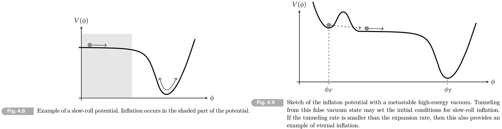
The simplest models of inflation implement the time-dependent dynamics during inflation in terms of the evolution of a scalar field, 𝜙(𝑡, 𝐱), called the inflaton. [𝑡: time, 𝐱: position] Associated with each value is a potential energy density 𝑉(𝜙) (see Fig. 4.8) When the field changes with time then it it also carries a kinetic energy density 1/2 𝜙̇2. If the energy associated with the scalar field dominates the universe, then it sources the evolution of the FRW background. We want to determine under which conditions this can derive an inflationary expansion. [RE Wikipedia inflaton]
Let us begin with a scalar field in Minkowski space. Its action is [RE Wikipedia Scalar field theory]
(4.39) 𝑆 = ∫ d𝑡 d3𝑥 [1/2 𝜙̇2 - 1/2 (∇𝜙)2 - 𝑉(𝜙)],
where we have also included the gradient energy, 1/2 (∇𝜙)2, associated with a spatially varying field. To determine the equation of the scalar field, we consider the variation 𝜙 → 𝜙 + 𝛿𝜙. Under this variation, the action changes as [RE Wikipedia Hamilton's principle]
(4.40) 𝛿𝑆 = ∫ d𝑡 d3𝑥 [𝜙̇𝛿𝜙̇ - ∇𝜙 ⋅ 𝛿∇𝜙 - d𝑉/d𝜙 𝛿𝜙]
{= ∫ d𝑡 3𝑥 [-d/d𝑡 (1/2 𝜙̇2) 𝛿𝜙 -(-∇ ⋅ ∇𝜙 𝛿𝜙) - d𝑉/d𝜙 𝛿𝜙]}
(4.41) = ∫ d𝑡 d3𝑥 [-d𝜙̇/d𝑡 + ∇2𝜙 - d𝑉/d𝜙]𝛿𝜙
where we have integrated by parts and dropped a boundary term. If the variation around the classical field configuration, then the principle of least-action states that 𝛿𝑆 = 0. For this to be valid for an arbitrary field variation 𝑑𝜙, the expression in the square brackets in (4.41) must vanish:
(4.42) d𝜙̇/d𝑡 - ∇2𝜙 = -d𝑉/d𝜙
This is the Klein-Gordon equation.
It is straightforward to extend this analysis to the evolution in an expanding FRW spacetime. For simplicity we will ignore spatial curvature.Physical coordinates are related to comoving coordinates by the scale factor, 𝑎(𝑡)𝐱.Taking this into account, it is easy to guess that the generalization of the action (4.49) to an FRW background is
(4.43) 𝑆 = ∫ d𝑡 d3𝑥 𝑎3(𝑡) [1/2 ᾡ2 - 1/2𝑎2(𝑡) (∇𝜙)2 - 𝑉(𝜙)],
We are interested in the evolution of a homogeneous field configurations, 𝜙 = 𝜙(𝑡), in which case the action reduces to
(4.44) 𝑆 = ∫ d𝑡 d3𝑥 𝑎3(𝑡) [1/2 𝜙̇2 - 𝑉(𝜙)],
Performing the same variation of the action as before, we find
(4.45) 𝛿𝑆 = ∫ d𝑡 d3𝑥 𝑎3(𝑡) [𝜙̇𝛿𝜙̇ - 𝑑𝑉/𝑑𝜙 𝛿𝜙].
(4.46) = ∫ d𝑡 d3𝑥 [-d/d𝑡 (𝑎3𝜙̇) - 𝑎3 d𝑉/d𝜙]𝛿𝜙
and the principle of least action leads to the following Klein-Gordon equation
(4.47) d𝜙̇/d𝑡 + 3𝐻𝜙̇ = -d𝑉/d𝜙.
The expansion has introduced one new feature, the so-called Hubble frictionassociated with the term 3𝐻ᾡ. This friction will play a crucial role in the inflationary dynamics.
Let us now assume that this scalar field dominates the universe and determine its effect on the expansion.Given the form of the action in (4.44), it is natural to guess that the energy density is the sum of kinetic and potential energy densities
(4.48) 𝜌𝜙 = 1/2 𝜙̇2 + 𝑉(𝜙).
Taking the time derivative of the energy density, we find
(4.49) 𝜌̇𝜙 = (𝑑𝜙̇/𝑑𝑡 + 𝑑𝑉/𝑑𝜙)𝜙̇ = -3𝐻𝜙̇2,
where the Klein-Gordon equation (4.47) was used. Comparing this to the continuity equation, ῤ𝜙 = -3𝐻(𝜌𝜙 + 𝑃𝜙) we infer the pressure induced by the field is
(4.50) 𝑃𝜙 = 1/2 ᾡ2 - 𝑉(𝜙).
This pressure determines the acceleration of the expansion 𝑑𝑎̇/𝑑𝑡 ∝ -(𝜌𝜙 + 3𝑃𝜙). We see that the density and pressure are in general not related by a constant equation of state as for a perfect fluid. Notice that if the kinetic energy of the inflation is much smaller than its potential energy, then 𝑃𝜙 ≈ -𝜌𝜙. The inflationary potential then acts like a temporary cosmological constant, sourcing a period of exponential expansion.
Exercise 4.3 The action of scalar field in a general curved spacetime is
(4.51) 𝑆 = ∫ 𝑑4𝑥√(-𝑔) [-1/2 𝑔𝜇𝜈∂𝜇𝜙∂𝜈𝜙 - 𝑉(𝜙)],
where 𝑔 ≡ det 𝑔𝜇𝜈, It is easy to check that this reduces to (4.43) for a flat FRW metric. Under a variation of the (inverse) metric, 𝑔𝜇𝜈 → 𝑔𝜇𝜈 + 𝛿𝑔𝜇𝜈, the action changes
(4.52) 𝛿𝑆 = -1/2 ∫ 𝑑4𝑥√(-𝑔) 𝛵𝜇𝜈𝛿𝑔𝜇𝜈,
where 𝛵𝜇𝜈 is the energy-momentum tensor.
Show that the energy-momentum tensor for a scalar field is
(4.53) 𝛵𝜇𝜈 = ∂𝜇𝜙∂𝜈𝜙 - 𝑔𝜇𝜈(1/2 𝑔𝛼𝛽∂𝛼𝜙∂𝛽𝜙 + 𝑉(𝜙)).
and confirm that this leads to the expressions for 𝜌𝜙 and 𝑃𝜙 found above. Hints: We have to use that 𝛿√(-𝑔) = -1/2 √(-𝑔) (𝑔𝜇𝜈𝛿𝑔𝜇𝜈).
Show that the conservation of the energy-momentum tensor, ∇𝜇𝛵𝜇𝜈 = 0, implies the Klein-Gordon equation (4.47).
[Solution] Under a variation of the inverse metric, the given action changes as follow
(a) 𝛿𝑆 = ∫ d4𝑥 [𝛿√(-𝑔) (-1/2 𝑔𝛼𝛽∂𝛼𝜙∂𝛽𝜙 - 𝑉(𝜙)) - √(-𝑔) 1/2𝛿𝑔𝜇𝜈∂𝜇𝜙∂𝜈𝜙] = 1/2 ∫ d4𝑥 √(-𝑔) [𝑔𝜇𝜈(1/2 𝑔𝛼𝛽∂𝛼𝜙∂𝛽𝜙 + 𝑉(𝜙)) - ∂𝜇𝜙∂𝜈𝜙]𝛿𝑔𝜇𝜈,
where we used 𝛿√(-𝑔) = -1/2 √(-𝑔) (𝑔𝜇𝜈𝛿𝑔𝜇𝜈). Comparing this (4.52) we get
(b) 𝛵𝜇𝜈 = ∂𝜇𝜙∂𝜈𝜙 - 𝑔𝜇𝜈(1/2 𝑔𝛼𝛽∂𝛼𝜙∂𝛽𝜙 + 𝑉(𝜙).
Raising one index, this yield
(c) 𝛵𝜇𝜈 = 𝑔𝜇𝛼∂𝛼𝜙∂𝛽𝜙 - 𝛿𝜇𝜈(1/2 𝑔𝛼𝛽∂𝛼𝜙∂𝛽𝜙 + 𝑉(𝜙).
For a homogeneous field configuration 𝜙(𝑡), this takes the form of a perfect fluid
(d) 𝛵𝜇𝜈 = diag (-𝜌𝜙, 𝑃𝜙, 𝑃𝜙, 𝑃𝜙).
(e) 𝜌𝜙 = -𝛵00 = -𝑔00∂0𝜙∂0𝜙 + 𝛿00(1/2 𝑔00∂0𝜙∂0𝜙 + 𝑉(𝜙) = 1/2 ᾡ2 + 𝑉(𝜙). [with 𝑔00 = -1, ∂0 ≡ ∂/∂(-𝑡)]
(f) 𝑃𝜙 = 1/3 𝛵𝑖𝑖 = -1/3 𝛿𝑖𝑖 (1/2 𝑔00∂0𝜙∂0𝜙 + 𝑉(𝜙)) = 1/2 ᾡ2 - 𝑉(𝜙).
This confirms the expressions derived in the text. We can now compute the covariant derivative of (4.53 or c)
(g) ∇𝜇𝛵𝜇𝜈 = 𝑔𝜇𝛼𝑔𝜈𝛽∇𝜇(∂𝛼𝜙∂𝛽𝜙) - 𝑔𝜇𝜈∇𝜇(1/2 𝑔𝛼𝛽∂𝛼𝜙∂𝛽𝜙 + 𝑉(𝜙) = 𝑔𝜇𝛼𝑔𝜈𝛽[∂𝜇(∂𝛼𝜙∂𝛽𝜙) - (𝛤𝜌𝜇𝛼∂𝛽𝜙 + 𝛤𝜌𝜇𝛽∂𝛼𝜙)∂𝜌𝜙] - 𝑔𝜇𝜈(1/2 𝑔𝛼𝛽∂𝛼𝜙∂𝛽𝜙 + 𝑉(𝜙)).
Using that 𝑔0𝑖 = 0 and ∂𝑖𝜙 = 0, this expression simplifies to
(h) ∇𝜇𝛵𝜇𝜈 = 𝛿𝜈0∂0ᾡ2 + 𝛤0𝜇𝛼𝑔𝜇𝛼𝛿𝜈0ᾡ2 + 𝛤00𝛽𝑔𝜈𝛽ᾡ2 + 𝛿0𝜈∂0(-1/2 ᾡ2 + 𝑉(𝜙)).
Recall that the Christoffel symbols with two times indies vanish. This implies that 𝛤00𝛽 = 0 and 𝛤0𝜇𝛼 = 𝛤0𝑖𝑗𝑔𝑖𝑗 = 𝐻𝑔𝑖𝑗𝑔𝑖𝑗 = 3𝐻, so that
(i) ∇𝜇𝛵𝜇𝜈 = 𝛿𝜈0[2𝜙̇ d𝜙̇/d𝑡 + 3𝐻𝜙̇2 + (-𝜙̇ d𝜙̇/d𝑡 + 𝜙̇ d𝑉/d𝜙)] = 𝛿𝜈0𝜙̇(d𝜙̇/d𝑡 + 3𝐻𝜙̇ + d𝑉/d𝜙).
The conservation of the energy-momentum tensor, ∇𝜇𝛵𝜇𝜈 = 0, then implies the Klein-Gordon equation
(j) d𝜙̇/d𝑡 + 3𝐻𝜙̇ + d𝑉/d𝜙 = 0. ▮
4.3.2 Slow-Roll Inflation
The dynamics during inflation is then determined by a combination of the Friedmann and Klein Gordon equations
(4.54) 𝐻2 = 1/3𝑀𝑃𝑙2 [1/2 𝜙̇2 + 𝑉], [RE (2.136) and (4.48)]
(4.55) d𝜙̇/𝑑𝑡 + 3𝐻𝜙̇ = -d𝑉/d𝜙
These equations are coupled. The energy stored in the field determines the Hubble rate, [𝐻], which in turn induces friction and hence affects the evolution of the field. We would like to determine the precise conditions under which this feedback leads to inflation.
A slowly rolling field
First, (4.54) and (4.55) can be combined into an expression for the evolution of the Hubble parameter
(4.56) Ḣ = -1/2 𝜙̇2/𝑀𝑃𝑙2. [from (4.54), 2𝐻Ḣ = 1/3𝑀𝑃𝑙2 [𝜙̇ d𝜙̇/d𝑡 + d𝑉/d𝜙 𝜙̇] → Ḣ = 1/6𝐻Ḣ𝑀𝑃𝑙2 [𝜙̇ d𝜙̇/d𝑡 - (d𝜙̇/d𝑡 + 3𝐻𝜙̇)𝜙̇] = -1/2 𝜙̇2/𝑀𝑃𝑙2.]
Talking the ratio of (4.56) and (4.54), we then find
(4.57) 𝜀 ≡ -Ḣ/𝐻2 = (1/2 𝜙̇2)/𝑀𝑃𝑙2𝐻2 = (3/2 𝜙̇2)/(1/2 𝜙̇2 + 𝑉).
Inflation (𝜀 ≪ 1) therefore occurs if the kinetic energy density, 1/2 𝜙̇2, only makes a small contribution to the total energy density, 𝜌𝜙 = 1/2 𝜙̇2 + 𝑉. For obvious reasons, this situation is called slow-roll inflation.
In order for slow-roll behavior to persist, the acceleration of the scalar field also has to be small. To assess this, it is useful to define the dimensionless acceleration per Hubble time
(4.58) 𝛿 ≡ -(d𝜙̇/d𝑡)/𝐻𝜙̇.
When 𝛿 is small, the friction term in (4.55) dominates and the inflation speed is determined by the slope of the potential. As long as the inflation kinetic energy stays subdominant and the inflationary expansion continues. To see this more explicitly, we take the time derivative of (4.57),
(4.59) 𝜀̇ = 𝜙̇ (d𝜙̇/d𝑡)/𝑀𝑃𝑙2𝐻2 - 𝜙̇2Ḣ/𝑀𝑃𝑙2𝐻3,
and substitute it into (4.36):
(4.60) 𝜅 = 𝜀̇/𝐻𝜀 = 2 (d𝜙̇/d𝑡)/𝐻𝜙̇ - 2 Ḣ/𝐻2 = 2(𝜀 - 𝛿).
This shows that {𝜀,∣𝛿∣} ≪ 1 implies {𝜀,∣𝜅∣} ≪ 1. If both the speed and the acceleration of the inflation field are small, then the inflationary expansion will last for a long time.
Slow-roll approximation
Now, we will use these condition to simplify the equations of motion. This is called the slow-roll approximation.
First, we note that 𝜀 ≪ 1 implies 𝜙̇2 ≪ 𝑉, which leads to the following simplification of Friedmann equation (4.54)
(4.61) 𝐻2 ≈ 𝑉/3𝑀𝑃𝑙2.
Next, we see that the condition ∣𝛿∣ ≪ 𝑉 simplifies the Klein-Gordon equation (4.55) to
(4.62) 3𝐻𝜙̇ ≈ -𝑉,𝜙,
where 𝑉,𝜙 ≡ d𝑉/d𝜙. This provides a simple relationship between the slope of the potential and the speed of the inflation. Finally, substituting (4.61) and (4.62) into (4.57) gives
(4.63) 𝜀 = (1/2 𝜙̇2)/3𝑀𝑃𝑙2𝐻2 ≈ 𝑀𝑃𝑙2/2 (-𝑉,𝜙/𝑉),
which express the parameter 𝜀 purely in terms of the potential.
To evaluate the parameter 𝛿 in (4.58), in the slow-roll approximation, we take the time derivative of (4.62), 3Ḣ𝜙̇ + 3𝐻d𝜙̇/d𝑡 = -𝑉,𝜙𝜙ᾡ. This leads to
(4.64) 𝜂 ≡ 𝛿 + 𝜀 = -(d𝜙̇/d𝑡
)/𝐻𝜙̇ -Ḣ/𝐻2 ≈ 𝑀𝑃𝑙2 𝑉,𝜙𝜙/𝑉.
Hence, a convenient way to judge whether a given potential 𝑉(𝜙) can leads to slow-roll inflation is to compute the potential slow-roll parameters
(4.65) 𝜀𝑉 ≡ 𝑀𝑃𝑙2/2 (𝑉,𝜙/𝑉)2, 𝜂𝑉 ≡ 𝑀𝑃𝑙2 𝑉,𝜙𝜙/𝑉.
Successful inflation occurs when these parameters are much smaller than unity.
Exercise 4.4 Show that in the slow-roll regime, the potential slow-roll parameters and the Hubble slow-roll parameters are related as follows:
(4.66) 𝜀𝑉 ≈ 𝜀 and 𝜂𝑉 ≈ 2𝜀 - 1/𝜅.
[Solution] In the slow-roll approximation, the Friedmann and Klein-Gordon equations are
(a) 𝐻2 ≈ 𝑉/3𝑀𝑃𝑙2, 3𝐻𝜙̇ ≈ -𝑉,𝜙
(b) 𝜀 = (1/2 𝜙̇2)/3𝑀𝑃𝑙2𝐻2 ≈ 𝑀𝑃𝑙2/2 (-𝑉,𝜙/𝑉), 𝜅 = 𝜀̇/𝐻𝜀 = 2 (d𝜙̇/d𝑡)/𝐻𝜙̇ - 2 Ḣ/𝐻2 = 2(𝜀 - 𝛿), 𝛿 ≡ -(d𝜙̇/d𝑡)/𝐻𝜙̇.
In the slow-roll approximation we have
(c) 𝛿 + 𝜀 = --(𝑑𝜙̇/𝑑𝑡)/𝐻𝜙̇ - -Ḣ/𝐻2 ≈ 𝑀𝑃𝑙2 𝑉,𝜙𝜙/𝑉 ≡ 𝜂𝑉
and hence
(d) 𝜀𝑉 ≈ 𝜀, 𝜂𝑉 ≈ 𝛿 + 𝜀 = -(𝜅/2 - 𝜀) + 𝜀 = 2𝜀 - 1/2 𝜅. ▮
The total number of 𝑒-foldings of accelerated expansion is
(4.67) 𝑁tot ≡ ∫𝑎𝑖𝑎𝑒 𝑑 ln 𝑎 = ∫𝑡𝑖𝑡𝑒 𝐻(𝑡) d𝑡 = ∫𝜙𝑖𝜙𝑒 𝐻/𝜙̇ 𝑑𝜙,
where 𝑡𝑖 and 𝑡𝑒 are defined as the time when 𝜀(𝑡𝑖) = 𝜀(𝑡𝑒) ≡ 1. In the slow-roll regime, we can use (4.63) to write the integral over the field space as
(4.68) 𝑁tot ≈ ∫𝜙𝑖𝜙𝑒 1/√(2𝜀𝑉) ∣𝑑𝜙∣/𝑀𝑃𝑙,
where 𝜙𝑖 and 𝜙𝑒 are the field values at the boundaries of the interval where 𝜀𝑉 < 1. As we have seen above, a solution to the horizon problem requires 𝑁tot ≳ 60, which provide an important constraint on successful inflation models.
Case study: quadratic inflation
As an example, let us give the slow-roll analysis of arguably the simplest model of inflation: single-field inflation driven by a mass term
(4.69) 𝑉(𝜙) = 1/2 𝑚2𝜙2.
As we will see in Chapter 8, this models is ruled out by CMB observation, but it still provides a useful example to illustrate the mechanism of slow-roll inflation. The slow-roll parameter for the potential are
(4.70) 𝜀𝑉(𝜙) = 𝜂𝑉(𝜙) = 2 (𝑀𝑃𝑙/𝜙)2.
To satisfy the slow-roll conditions {𝜀𝑉, ∣𝜂𝑉∣} < 1, we need to consider super-Planckian value for the inflation
(4.71) 𝜙 > √2𝑀𝑃𝑙 ≡ 𝜙𝑒.
Let the initial field value be 𝜙𝑖, The 𝑒-foldings of inflationary expansion are
(4.72) 𝑁tot = ∫𝜙𝑖𝜙𝑒 d𝜙/𝑀𝑃𝑙 1/√(2𝜀𝑉) = 𝜙2/4𝑀𝑃𝑙2∣𝜙𝑒𝜙𝑖 = 𝜙𝑖2/4𝑀𝑃𝑙2 - 1/2.
To obtain 𝑁tot > 60, the initial field value must satisfy
(4.73) 𝜙𝑖 > 2√60 𝑀𝑃𝑙 ~ 15𝑀𝑃𝑙.
We note that the total field excursion is super-Planckian, ∆𝜙 = 𝜙𝑖 - 𝜙𝑒 ≫ 𝑀𝑃𝑙. In Section 4.4.1, we will discuss whether this large field variation should be a cause for concern.
4.3.3 Creating the Hot Universe
Most of the energy density during inflation is the form of the inflaton potential 𝑉(𝜙). Inflation ends when the potential sleeps and the field picks up kinetic energy. The energy in the inflation sector then has to transferred to the particles of the Standard Model. This process is called reheating and starts the hot BB.
Once the inflation field reaches the bottom of the potential, it begins to oscillate. Near the minimum, the potential can be approximated as 𝑉(𝜙) ≈ 1/2 𝑚2𝜙2 and the equation of motion of the inflation is
(4.74) d𝜙̇/d𝑡 + 3𝐻𝜙̇ = -𝑚2𝜙. [RE (4.47) ]
The energy density evolves according to the continuity equation [RE (4.50) (4.69)]
(4.75) 𝜌̇𝜙 + 3𝐻𝜌𝜙 = -3𝐻𝑃𝜙 = 3/2 𝐻 (𝑚2𝜙2 - ᾡ2),
where the right-hand side averages to zero over one oscillation period. This averaging has ignored the Hubble friction in (4.74), which is justified on timescales shorter than the expansion time. The oscillating field behaves like pressureless matter, with 𝜌𝜙 ∝ 𝑎-3 (See problem 4.1 for the derivation). As the energy density drops, the amplitude of the oscillation decreases.
To avoid that the universe ends up completely empty, the inflaton has to couple to Standard Model fields. The energy stored in the inflaton filed will then be transferred to ordinary particles. If the decay is slow, then the inflaton's energy density follows the equation
(4.76) 𝜌̇𝜙 + 3𝐻𝜌𝜙 = -𝛤𝜙𝜌𝜙,
where 𝛤𝜙 parameterizes the inflaton decay rate. A slow decay of the inflaton typically occurs if the coupling is only to fermions. If the inflaton can also decay into bosons then the decay rate may be enhanced by Bose condensation and parametric resonance effects. This kind of rapid decay is called preheating, since the bosons are created far from thermal equilibrium.
the new particles will interact with each other and eventually reach the thermal state that characterizes the hot Big Bang. The energy density at the end of reheating epoch is 𝜌𝑅 < 𝜌𝜙,𝑒 is the energy density at the end of inflation, and reheating temperature 𝛵𝑅 is determined by
(4.77) 𝜌𝑅 = π2/30 𝑔*(𝛵𝑅) 𝛵𝑅4.
If reheating takes a long time, then 𝜌𝑅 ≪ 𝜌𝜙,𝑒 and the reheating temperature gets smaller. At a minimum, the reheating temperature has to be larger than 1 MeV to allow for successful BBN, and most likely it is much larger than this to also allow for baryongenesis after inflation.
This completes our highly oversimplified sketch of the reheating phenomenon. In reality, the dynamics during reheating can be very rich, often involving non-perturbative effects captured by numerical simulation (for review see [2-5]). Describing this phase in the history is essential for understanding how the hot Big Bang began.With accelerated expansion having ended, there is no "cosmic amplifier" to make the microscopic physics of reheating easily accessible on cosmological length scales. Moreover, the high energy scale associated with the end of inflation, as well as the subsequent thermalization, can further hide details of this era from our low-energy probes. Nevertheless, in some cases, the dynamics during this period can generate relics such as isocurvature perturbations, stochastic gravitational waves, non-Gaussianities, dark matter/radiation, primordial black holes, topological and non-topological solitons, matter/antimatter asymmetry, and primordial magnetic fields. Detecting any of these relics would give us an interesting window into the reheating era.
4.4 Open Problems*
Despite its phenomenological success, inflation is not yet a complete theory. To achieve inflation we had to postulate new physics at energies far above those probed by particle colliders and its success is sensitive to assumption about the physics at even higher energies.
4.4.1 Ultraviolet Sensitivity
The most conservative way to describe the inflationary era is in terms of an effective field theory (EFT). In the EFT approach, we admit that we don't know the details of the high-energy theory and instead parameterize our ignorance. We begin by defining the degrees of freedom and symmetries of the inflationary theory. This theory is valid below a cutoff scale 𝛬, and we should ask how the unknown physics above the scale 𝛬 can affect the low-energy dynamics during inflation. This means writing down all possible corrections to the low-energy theory that are consistent with the assume symmetries. The effective Lagrangian of the theory can then be written as
(4.78) 𝓛eff[𝜙] = 𝓛0[𝜙] + ∑𝑛 𝑐𝑛 𝑂𝑛[𝜙]/𝛬𝛿𝑛 - 4,
where 𝓛0 is the Lagrangian of the inflationary model and 𝑂𝑛 are a set of "operators" that parameterize the corrections coming from the couplings to additional high-energy degrees of freedom. The dimensionless parameters 𝑐𝑛 are usually taken to be of order one.8 If the cutoff scale 𝛬 is much larger than the typical energy 𝐸 at which the low-energy theory is being probed, then the corrections are small, suppressed by powers of 𝐸/𝛬. This is why quantum gravity doesn't affect our everyday lives, or even those of our friends working at particle colliders.9 A remarkable feature of inflation, however, is that it is extremely sensitive even to effects suppressed by the Planck scale.
We have seen that slow-roll inflation requires a flat potential (in Planck scale), but his is hard to control and sensitive to very small corrections. In the absence of any special symmetries, the EFT of slow-roll inflation takes the following form
(4.79) 𝓛eff[𝜙] = -1/2 (𝜕𝜇𝜙)2 - 𝑉(𝜙) - ∑𝑛 𝑐𝑛 𝑉(𝜙) 𝜙2𝑛/𝛬4𝑛 + ∙ ∙ ∙ ,
where a representative set of higher-dimension operators is written. If the inflation field value is smaller than the cutoff scale we can truncate the 𝐸𝐹𝛵 expansion in (4.79) and the leading effect comes from the dimension-six operator
(4.80) ∆𝑉 = 𝑐1𝑉(𝜙) 𝜙2/𝛬2.
Since 𝜙 ≪ 𝛬, this is a small correction to the inflation potential, ∆𝑉 ≪ 𝑉. Nevertheless, it affects the delicate flatness of the potential and hence is relevant for the dynamics during inflation. In particular, the slow-roll parameter 𝜂𝑉 receives the correction
(4.81) ∆𝜂𝑉 = 𝑀𝑃𝑙2/𝑉 (∆𝑉),𝜙𝜙 ≈ 2𝑐1 (𝑀𝑃𝑙/𝛬)2 > 1,
where the final inequality comes from 𝑐1 = 𝑂(1) and 𝛬 < 𝑀𝑃𝑙. Notice that this problem is independent of the energy scale of inflation. All inflationary models have to address this so-called eta problem.
One promising way to solve the eta problem is to postulate a shift symmetry for he inflation, 𝜙 → 𝜙 + 𝑐, where 𝑐 is constant. If this symmetry is respected by the couplings to massive fields, then having 𝑐𝑛 ≪ 1 is technically natural [6]. Another way to ameliorate the eta problem is supersymmetry. Above the scale 𝐻, the theory is supersymmetric and the contribution from bosons and fermions precisely cancel as a minor miracle. However, supersymmetry is spontaneously broken during inflation, leading yo an inflaton mass of order the Hubble scale, 𝑚𝜙 ~ 𝐻, and an eta parameter of order one, ∆𝜂𝑉 ~ 1. Although the eta problem is still there, it is much less severe and requires just a percent-level fine-tuning of inflaton mass parameter.
We have seen that in quadratic inflation the inflaton moves over a super-Planckian distance in field space, ∆𝜙 > 𝑀𝑃𝑙. This is a general feature of all inflationary models with observable gravitational wave signals. The sper-Planckian excursion of the field should make us nervous. When the field value isn't smaller than the cutoff, we cannot trust the EFT expansion in (4.79). Models of large-field inflation therefore usually invoke symmetries-such as an approximate shift symmetry 𝜙 → 𝜙 + 𝑐-to suppress the couplings of the inflaton to massive degree off freedom and reduce the size of the corrections in (4.79). An important question is whether the assumed symmetries are respected by the UV-completion.
The UV sensitivity of inflation is a challenge, because we either need to work in a UV-complete theory of quantum gravity or make assumptions about the form that such a UV-completion might take. It is also an opportunity,, because it suggests the exciting possibility of using cosmological observations to learn about fundamental aspects of quantum gravity [7].
4.4.2 Initial Conditions
First, Imagine that the inflation field initially takes different values in different regions of space, some at top of the potential, some at the bottom. The regions of space with large vacuum energy will inflate and grow. Weighted by volume, these regions will dominate, explaining why most f space experience inflation. Alternatively, it is sometimes assumed that slow-roll inflation was proceeded by an earlier phase of false vacuum domination (see Fig. 4.9. In quantum mechanics, there is a small probability that the field will tunnel through the potential energy barrier. so the question becomes why the quantum mechanical tunneling is more likely to put the inflaton field at the top of the potential than at its minimum. We should still ask why the universe started in the high-energy false vacuum. Most ambitiously, the no-boundary proposal by Hartle and Hawking gives a prescription for evaluating the provability that a universe is spontaneously created from nothing [8].
Second, if the initial inflaton velocity is non-negligible, then it is possible that the field will overshoot the region of the potential where inflation is supposed to occur, without actually sourcing accelerated expansion. In small-field models the Hubble friction is often not efficient enough to slow down the field before it reaches the region of interest. But in large-field models, on the other hand, Hubble friction is usually very efficient and the slow-roll solution becomes an attractor.
Finally, since inflation is supposed to explain the homogeneous initial conditions of the hot BB, we must ask what happens when allow for large inhomogeneities in the inflaton field, These inhomogeneities carry gradient energy, which might hinder the accelerated expansion. The sensitivity of an inflationary model to initial perturbations of the inflaton field is best addressed by numerical simulations. In 1989 the earliest such simulations were performed in 1 + 1 dimensions [9, 10]. Recently the problem was revisited using simulation in 3 + 1 dimensions [11, 12]. It was again found that large-field models are more robust than small-field models.
4.4.3 Eternal Inflation
A rather dramatic consequence of the quantum dynamics of inflation may be that globally that it never ends, but is eternal. There are two types of eternal inflation, both are illustrated in Fig. 4.9. First, inflation can occur while the field is stuck in false vacuum. Any region of space has a finite probability to decay and reach the true vacuum via quantum tunneling. If the decay rate is 𝛤, then the probability that the region will survive in the inflationary state is 𝑒-𝛤𝑡. The volume of inflating region increases as 𝑒3𝑡. If the rate of exponential expansion is larger than the rate of decay, then inflation does not end globally. There are many pockets of space where inflation does end-one of these pockets is so-called our "universe"-but they are embedded in a much larger "multiverse." The space between the pocket universes is rapidly expanding, creating new space, where new pocket universes can form. This never ends.
We will study the effects of quantum mechanics on the dynamics of inflation and see that the field experiences random fluctuations up and down the potential. Eternal inflation occurs if these quantum fluctuation dominate over the classical rolling. Consider the evolution of the field in one Hubble volume 𝐻-3 during one Hubble time ∆𝑡 = 𝐻-1. Classically, the field will change by ∆𝜙𝑐𝑙 ~ ᾡ𝐻-1. At the same time, quantum mechanics induces random jitters ∆𝜙𝑄, so that the total change of the field is
(4.82) ∆𝜙 = ∆𝜙𝑐𝑙 + ∆𝜙𝑄.
How big does this probability have to be in order for inflation to be eternal? During a Hubble time, the volume increases by a factor of 𝑒3 ≈ 20, meaning that the inflationary region breaks up into 20 Hubble-sized regions. As we will see in Chapter 8, averaged over one of these 20 regions, inflationary quantum fluctuations have a Gaussian probability distribution with width 𝐻/2π. If the probability to have ∆𝜙 < 0 is greater than 1 in 20, then the volume of space that is inflating will increase. When
(4.83) ∆𝜙𝑄 = 𝐻/2π > 0.6 ∆𝜙𝑐𝑙 = 0.6 ∣𝜙̇∣𝐻-1.
If the condition is satisfied, inflation will continue forever, This arguments for slow-roll eternal inflation was admittedly somewhat heuristic and it is sill being debated the reliability.
Exercise 4.5 Show that, in quadratic inflation, slow-roll eternal inflation occurs for
(4.84) 𝜙2/𝑀𝑃𝑙2 ≳ 13 𝑀𝑃𝑙/𝑚. [verification needed]
In Chapter 8, we will find that in order for the predicted CMB fluctuations to have the right amplitude, we must have 𝑚 ~ 10-6 𝑀𝑃𝑙. This implies 𝜙 > 3600 𝑀𝑃𝑙. In that case the regime of eternal inflation would not exist. [verification needed]
[Solution] The condition for eternal inflation is and assuming a quadratic potential 𝑉(𝜙) = 𝑚2𝜙2/2
(a) ∆𝜙𝑄 = 𝐻/2π > 0.6 ∆𝜙𝑐𝑙 = 0.6 ∣𝜙̇∣𝐻-1 ⇒ 𝐻2 > 0.6 × 2π∣𝜙̇∣ ≈ 3.8∣𝜙̇∣
(b) 𝐻2 ≈ 𝑉/3𝑀𝑃𝑙2 = 𝑚2𝜙2/3𝑀𝑃𝑙2
(c) ∣𝜙̇∣ ≈ ∣𝑉,𝜙∣/3𝐻 ≈ √3𝑀𝑃𝑙∣𝑉,𝜙∣/3√𝑉 = 𝑀𝑃𝑙 𝑑(𝑚2𝜙2/2)/d𝜙 × 1/[√(3/2)𝑚𝜙] = √(2/3) 𝑚𝑀𝑃𝑙.
The condition 𝐻2 > 3.8∣𝜙̇∣ implies
(d) 𝑚2𝜙2/3𝑀𝑃𝑙2 > 3.8√(2/3)𝑚𝑀𝑃𝑙 ⇒ 𝜙2/𝑀𝑃𝑙2 > 6/𝑚2 × 3.8√(2/3)𝑚𝑀𝑃𝑙 = 3.8√24 𝑀𝑃𝑙/𝑚 ≈ 18.6 𝑀𝑃𝑙/𝑚. [verification needed]
Using 𝑚 ~ 10-6𝑀𝑃𝑙, this implies 𝜙 > 4300 𝑀𝑃𝑙. ▮ [verification needed]
The concept of eternal inflation is almost as old as inflation itself, it recently revived in the context of string theory. the string theory seems to give rise to a large number of metastable solutions.The space vacua is called the string landscape. The physics may be different in each of these vacua. Eternal inflation provides the mechanism by which this landscape populated. The fact that eternal inflation combined with the string landscape allows for a solution the the cosmological constant problem (see Section 2.3.3) is the single most important reason to take either of these ideas seriously.
Let us finally address the elephant in the room: the measure problem of the inflationary multiverse. We have seen that eternal inflation produces an infinite number of universe. The fraction of universes with a certain observable property is equal to infinity divided by infinity. Unfortunately, the answer tends to depend sensitively on type of regulator that is being used.
Although we have remarkable observational evidence that something like inflation occurred in the early universe (see Chapter 8), inflation cannot yet be considered a part of the standard model of cosmology, Inflation is still a work in progress.
4.5 Summary
In this chapter, we have studied inflation. We stared with a discussion of the causality problems of the hot BB, highlighting the crucial role played by the evolution of the comoving Hubble radius, (𝑎𝐻)-1. We showed that this evolution determines the particle horizon-the maximal distance that light can propagate between an initial time 𝑡𝑖 and a later time 𝑡:
(4.85) d𝘩(𝜂) = ∫𝑡𝑖𝑡 d𝑡/𝑎(𝑡) = ∫𝑁𝑖𝑁 (𝑎𝐻)-1 d𝑁,
where 𝑁 = ln 𝑎.Since the comoving Hubble radius is monotonically increasing in the conventional BB theory, the particle horizon is dominated by the contributions from late times. Most parts of the CMB would then never have been causal contact, yet they have nearly the same temperature. This is the horizon problem.
Inflation is a period of accelerated expansion during which the comoving Hubble radius is shrinking. The particle horizon receives most of its contribution from early times and can be much larger than naively assumed. Causal contact is established in the time before the hot BB. The shrinking of the comoving Hubble radius also solves the closely related flatness problem and allows a causal mechanism to generate superhorizon correlations.
Inflation occurs if all physical quantities vary slowly with time. For example, the fractional change of the Hubble rate during inflation must be small,
(4.86) 𝜀 ≡ -Ḣ/𝐻2 ≪ 1.
To solve the problems of the ht BB, this condition must be maintained for about 60 𝑒-foldings of expansion. A popular way to achieve this is through a slowly rolling scalar field (the inflaton). The evolution of the inflaton is governed by the Klein-Gordon equation
(4.87) d𝜙̇/d𝑡 + 3𝐻𝜙̇ = -𝑉,𝜙.
The field rolls slowly if the dynamics is dominated by the friction term, ∣d𝜙̇/d𝑡∣ ≪ ∣3𝐻𝜙̇∣ ≈ ∣𝑉,𝜙∣. The size of the friction is determined by the energy density associated with the inflation itself, which by the Friedmann equation determines the expansion rate
(4.88) 𝐻2 = 1/3𝑀𝑃𝑙2 [1/2 𝜙̇2 + 𝑉].
Inflation requires that the kinetic energy is much smaller than the potential energy, 1/2 ᾡ2 ≪ 𝑉. The conditions for successful slow-roll inflation can be characterized by the slow-roll parameters
(4.89) 𝜀𝑉 ≡ 𝑀𝑃𝑙2/2 (𝑉,𝜙/𝑉)2, 𝜂𝑉 ≡ 𝑀𝑃𝑙2 𝑉,𝜙𝜙/𝑉.
Inflation will occur in regions of potential where {𝜀𝑉, ∣𝜂𝑉∣} ≪ 1. Achieving such flat potentials in a theory of quantum gravity is challenging.
7 This parameter is often denoted 𝜂. the parameter 𝜀 and 𝜅 are often called Hubble slow-roll parameters to distinguish potential slow-roll parameters defined in Section 4.3.1.
8 Some new degrees of freedom must appear below the Planck scale, 𝛬 ≲ 𝑀𝑃𝑙, because gravity is not renormalizable and needs a high-energy (or "ultraviolet") completion. If 𝜙 has order-one couplings to any heavy fields, with masses of order 𝛬, then integrating out these fields yields the effective action (4.78), with order-one couplings 𝑐𝑛.
9 Note that the largest energies proved at the Large Hadron Collier (LHC) are still tiny relative to the Planck scale, 𝐸/𝑀𝑃𝑙 < 10-16.
Problems
4.1 Oscillating scalar field
The action for a scalar field in a curved space time is
(a) 𝑆 = ∫ d4 𝑥√(-𝑔) [-1/2 𝑔𝜇𝜈∂𝜇𝜙∂𝜈𝜙 - 𝑉(𝜙)],
where 𝑔 ≡ det 𝑔𝜇𝜈 is the determinant of the metric tensor.
1. Evaluate the action for the homogeneous field 𝜙 = 𝜙(𝑡) in a flat FRW spacetime and determine the equation of the motion for the field.
[Solution] For the FRW metric,
(b) d𝑠2 = -d𝑡2 + 𝑎2(𝑡) d𝐱2.
the determinant of the matrix, 𝑔𝜇𝜈 = diag (-1, 𝑎2, 𝑎2, 𝑎2), is 𝑔 = -𝑎6(𝑡). The scalar field is constrained by the symmetries of the FRW spacetime to evolve over only in time 𝜙(𝑡, 𝐱) = 𝜙(𝑡). The Lagrangian in the example is then
(c) 𝐿 = 𝑎3[1/2 𝜙̇2 - 𝑉(𝜙)]
We use the Euler-Lagrange equation
(d) d/d𝑡 (∂𝐿/∂𝜙̇) - ∂𝐿/∂𝜙 = 0, ∂𝐿/∂𝜙̇ = 𝑎3𝜙̇, ∂𝐿/∂𝜙 = -𝑎3∂𝑉/∂𝜙.
(e) d/d𝑡 (𝑎3𝜙̇) = 3𝑎2 d𝑎/d𝑡 𝜙̇ + 𝑎3d𝜙̇/d𝑡
(f) 𝑎3(3𝑎̇/𝑎 𝜙̇ + d𝜙̇/d𝑡 + d𝑉/d𝜙) = 𝑎3(3𝐻𝜙̇ + d𝜙̇/d𝑡 + d𝑉/d𝜙) = 0.
Substituting this into (d), we get
(g) d𝜙̇/d𝑡 + 3𝐻𝜙̇ = -d𝑉/d𝜙. [(4.47) Klein-Gordon equation] ▮
|
|
|