|
김관석
|
2024-12-22 21:43:08, 조회수 : 54 |
- Download #1 : BC_8b.jpg (124.0 KB), Download : 0

8.2 Quantum Fluctuations
As we have just seen, the Fourier modes of the field fluctuations satisfy the equation of motion of a harmonic oscillator. In this section the quantization of these oscillators will be described.
8.2.1 Quantum Harmonic Oscillators
We first study the simple case of a 1-dimensional harmonic oscillator in quantum mechanics. Consider a mass 𝑚 attached to a spring with spring constant 𝜅. Let 𝑞 be the deviation from the equilibrium point, whose equation is d2𝑞/dt2 = - 𝜔2𝑞, where 𝜔 ≡ √(𝜅/𝑚)* is the oscillation frequency. [*correction: 𝜔2 ≡ √(𝜅/𝑚) in the text → 𝜔 ≡ √(𝜅/𝑚)]. The quantization of the oscillator is a textbook problem in quantum mechanics. [RE Wikipedia Quantum harmonic oscillator]
The Hamiltonian of the oscillator is
(8.30) 𝐻 = 1/2 𝑝2 + 1/2 𝜔2𝑞2,
where we rescaled the amplitude to set 𝑚 ≡ 1and introduced the conjugate momentum 𝑝 ≡ 𝑞̇. Finding the spectrum energy eigenstates of this Hamiltonian, we promote 𝑝 and 𝑞 to quantum operator 𝑝̂ and 𝑞̂ and impose the canonical commutation relation
(8.31) [𝑞̂, 𝑝̂] ≡ 𝑞̂𝑝̂ - 𝑝̂𝑞̂ = 𝑖ℏ,
where ℏ is the reduced Planck constant. An elegant way to solve for the spectrum of states is to express 𝑞̂ and 𝑝̂ in term of annihilation and creation operators (ladder operators in some textbooks) :
(8.32) 𝑞̂ = √(ℏ/2𝜔) (𝑎̂ + 𝑎̂†), 𝑝̂ = -𝑖√(ℏ𝜔/2) (𝑎̂ - 𝑎̂†),
where the commutation relation (8.31) is satisfied if
(8.33) [𝑎̂, 𝑎̂†] = 1.
The Hamiltonian (8.30) can then be written as
(8.34) 𝐻̂ = 1/2 𝑝̂2 + 1/2 𝜔2𝑞̂2 = 1/2 ℏ𝜔(𝑎̂𝑎̂† + 𝑎̂†𝑎̂) = ℏ𝜔(𝑎̂𝑎̂† + 1/2).
The ground state of the oscillator is defined by
(8.35) 𝑎̂∣0⟩ = 0,
and has energy 𝐸0 ≡ ⟨0∣𝐻̂∣0⟩ = 1/2 ℏ𝜔. Excited states are construct by repeated application of the creation operator
(8.36) 𝑎̂∣𝑛⟩ = 1/√𝑛! (𝑎̂†)𝑛∣0⟩,
and have energy 𝐸𝑛 ≡ ⟨𝑛∣𝐻̂∣𝑛⟩ = ℏ𝜔(𝑛 + 1/2).
The expectation value of the position operator 𝑞̂ in the ground states ∣0⟩ vanishes,
(8.37) ⟨𝑞̂⟩ ≡ ⟨0∣𝑞̂∣0⟩ = √(ℏ/2𝜔) ⟨0∣𝑎̂ + 𝑎̂†∣0⟩ = 0,
because 𝑎̂ annihilates ∣0⟩ when acting on it from the left, and 𝑎̂† annihilates ⟨0∣ when acting on it from the right. However the expectation value of the square of the position operator receives finite zero-point fluctuations:
(8.38) ⟨∣𝑞̂∣2⟩ ≡ ⟨0∣𝑞̂†𝑞̂∣0⟩ = ℏ/2𝜔⟨0∣(𝑎̂† + 𝑎̂)(𝑎̂ + 𝑎̂†)∣0⟩ = ℏ/2𝜔⟨0∣𝑎̂𝑎̂†∣0⟩ = ℏ/2𝜔⟨0∣[𝑎̂, 𝑎̂†] + 𝑎̂†𝑎̂∣0⟩ = ℏ/2𝜔 ⟨0∣[𝑎̂, 𝑎̂†]∣0⟩ = ℏ/2𝜔.
These zero-point fluctuations play an important role in many areas of physics and, in particular, seem to be the origin of all structure in the universe.
Uncertainty principle A heuristic way to derive the result (8.38) is from the uncertainty principle
(8.39) ∆𝑞̂∆𝑝̂ = ℏ/2,
where ∆𝑞̂ and ∆𝑝̂ are the uncertainties in the position and momentum of the oscillator, respectively. The energy of the quantum harmonic oscillator due to these quantum fluctuation the is
(8.40) 𝐸 = ℏ2/8(∆𝑞̂)2 + 1/2 𝜔2(∆𝑞̂)2.
This energy is minimized for
(8.41) d𝐸/d(∆𝑞̂)2) = - ℏ2/8(∆𝑞̂)4 + 1/2 𝜔2 = 0 ⇒ ∆𝑞̂ = √(ℏ/2𝜔),
reproducing our previous result (8.38). Substituting his back into (8.40) gives 𝐸0 = 1/2 ℏ𝜔, the zero-point energy of the oscillator in the ground state. ▮
The only subtlety for applying it to inflation will be that the frequency of the oscillations is time dependent, 𝜔 = 𝜔(𝑡). It is most convenient to describe this time dependence in the Heisenberg picture where operators vary in time , while states are time independent. An operator 𝑂̂ in the Heisenberg picture satisfies the following equation:
(8.42) d𝑂̂/d𝑡 = 𝑖/ℏ [𝐻̂, 𝑂̂],
where 𝐻̂ is the Hamiltonian.
Exercise 8.5 Applying (8.42) to the operators 𝑞̂ and 𝑝̂, show that
(8.42) d2𝑞̂/d𝑡2 + 𝜔2𝑞̂ = 0,
i.e. the quantum operator 𝑞̂ obeys the same equation of motion as classical variable 𝑞.
[Solution] According to Heisenberg picture equation we have
(a) d𝑞̂/d𝑡 = 𝑖/ℏ [𝐻̂, 𝑞̂], d𝑝̂/d𝑡 = 𝑖/ℏ [𝐻̂, 𝑝̂]
Since 𝐻̂ = 1/2 𝑝̂2 + 1/2 𝜔2𝑞̂
(b) [𝐻̂, 𝑞̂] = 1/2 [𝑝̂2, 𝑞̂] = [𝑝̂, 𝑞̂] 𝑝̂ = -𝑖ℏ 𝑝̂,
(c) [𝐻̂, 𝑝̂] = 1/2 𝜔2[𝑞̂2, 𝑝̂] = 𝜔2[𝑞̂, 𝑝̂] 𝑞̂ = 𝑖ℏ𝜔2 𝑞̂, So we get
(d) d𝑞̂/d𝑡 = 𝑝̂, d𝑝̂/d𝑡 = -𝜔2𝑞̂,
Hence we find
(e) d2𝑞̂/d𝑡2 + 𝜔2𝑞̂ = 0. ▮
We now write the position operator as
(8.44) 𝑞̂ = 𝑞(𝑡)𝑎̂(𝑡𝑖) + 𝑞*(𝑡)𝑎̂†(𝑡𝑖),
where the complex mode function 𝑞(𝑡) satisfies d2𝑞/d𝑡2 + 𝜔2(𝑡)𝑞 = 0. The annihilation operator 𝑎̂(𝑡𝑖)-and hence the associated vacuum state ∣0⟩-depends on the time 𝑡𝑖 at which it is defined. In the inflationary application, there will be preferred moment at which we define the vacuum state, namely the beginning of inflation.
Substituting (8.44) into (8.31), we get
(8.45) [𝑞̂, 𝑝̂] = (𝑞𝑞̇* - 𝑞̇𝑞*) = 𝑖ℏ.
In order for this to give [𝑎̂, 𝑎̂†] = 1, we require the mode function to obey the normalization
(8.46) 𝑞𝑞̇* - 𝑞̇𝑞* = 𝑖ℏ.
To completely fix the mode function and hence give a unique meaning to the operator 𝑎̂(𝑡𝑖) and the corresponding vacuum state ∣0⟩, we need to impose a second condition on the solution 𝑞(𝑡).
As we saw in (8.25), at early times, the inflaton fluctuations satisfy the equation of motion of a harmonic oscillator with a fixed frequency. To model the situation during inflation, we consider a harmonic oscillator whose frequency initially a constant and then slowly develops a time dependence. We take the initial condition to be the ground state of the fixed -frequency oscillator (which will include the zero-point fluctuations discussed above) and then use the equation of motion with a time-dependent frequency to evolve these fluctuations forward in time.
To see how a preferred mode function arises for a harmonic oscillator with a fixed frequency, let us write the most general solution as
(8.47) 𝑞(𝑡) = 𝑟(𝑡)𝑒𝑖𝑠(𝑡),
where 𝑟(𝑡) and 𝑠(𝑡) are real functions of time, and (8.46) implies
(8.48) 𝑠̇ = - ℏ/2𝑟2.
We would like to determine the solution that minimizes the vacuum expectation value of the Hamiltonian
(8.49) ⟨0∣𝐻̂∣0⟩ = 1/2 (∣𝑞̇∣2 + 𝜔2∣𝑞∣2) = 1/2 (𝑟̇2 + 𝑟2𝑠̇2 + 𝜔2𝑟2).
Substituting (8.48), we get
(8.50) ⟨0∣𝐻̂∣0⟩ = 1/2 (𝑟̇2 + ℏ2/4𝑟2 + 𝜔2𝑟2).
This is minimized for 𝑟̇ = 0 and [If we apply d/d𝑟2 at both sides of equality, then we get]
(8.51) 0 = d/d𝑟2 (ℏ2/4𝑟2 + 𝜔2𝑟2) = -ℏ2/4(𝑟2)2 + 𝜔2 ⇒ 𝑟 = √(ℏ/2𝜔)
Substituting this back into (8.48), we find
(8.52) 𝑠̇ = -𝜔 ⇒ 𝑠 = -𝜔𝑡 + const.
Up to an irrelevant phase, we therefore get
(8.53) 𝑞(𝑡) = √(ℏ/2𝜔) 𝑒-𝑖𝜔𝑡 (𝜔 = const).
We see that the ground state corresponds to the positive-frequency solution, 𝑒-𝑖𝜔𝑡, while adding any amount of the negative frequency solution, 𝑒+𝑖𝜔𝑡, would raise the energy.
Using the solution (8.53) as an initial condition at 𝑡 = 𝑡𝑖 uniquely fixes the solution to d2𝑞/d𝑡2 = 𝜔2(𝑡)𝑞. Of course the explicit solution depends on 𝜔(𝑡), which in the case of inflation is determined by the evolution of the inflationary background. Repeating the manipulations that led to (8.38), we get that the variance of the position operator is simply the square of the mode function:
(8.54) ⟨∣𝑞̂∣2⟩ = ∣𝑞(𝑡)∣2.
This describes how the initial zero-point fluctuations, specified in (8.38), evolve in time.
8.2.2 Inflationary Vacuum Fluctuations
We are now ready to apply the quantization procedure to the field fluctuations during inflation. for simplicity, we will work in the slow-roll approximation, taking the background spacetime to be de Sitter space, with 𝐻 = const and 𝑎 = -(𝐻𝜂)-1,, The Mukhanov-Sasaki equation (8.18) then takes the form
(8.55) 𝑓𝐤ʺ + (𝑘2 - 2/𝜂2)𝑓𝐤 = 0.
In spatially flat gauge, this is a good approximation before horizon crossing. However on superhorizon scales slow-roll corrections are the leading effect. For example, ignoring the time dependence of expansion rate will lead to a fictitious evolution of the curvature perturbation 𝓡 on large scales. To minimize this error, we will evaluate all fluctuations at the moment of horizon crossing, 𝑘 = 𝑎𝐻, where we match them to the conserved curvature perturbation. Includinf a time-dependent expansion rate 𝐻(𝑡), in the horizon crossing condition then extends our results to a quasi-de Sitter background. We also include the weak time dependence in the conversion from 𝛿𝜙 to 𝓡 in (8.29). In turns out that this simple prescription gives the right answer, as we will prove later by a more rigorous treatment.
Canonical quantization
The quantization of the field fluctuation s is essentially the same as for the harmonic oscillator. We first promote the field 𝑓(𝜂, 𝐱) and its conjugate momentum 𝜋(𝜂, 𝐱) to quantum operators 𝑓̂(𝜂, 𝐱) and 𝜋̂(𝜂, 𝐱), and then impose
(8.56) [𝑓̂(𝜂, 𝐱), 𝜋̂(𝜂, 𝐱ʹ)] = 𝑖 𝛿𝐷(𝐱 - 𝐱ʹ),
where we set ℏ ≡ 1. This is the field theory equivalent of (8.31). The delta function enforces locality: modes at different points in space are independent and the corresponding operators therefore commute. In Fourier space, we find
(8.57) [𝑓̂(𝜂, 𝐱), 𝜋̂(𝜂, 𝐱ʹ)] = ∫ d3𝑥 ∫ d3𝑥ʹ [𝑓̂(𝜂, 𝐱), 𝜋̂(𝜂, 𝐱ʹ)] 𝑒-𝑖𝐤⋅𝐱𝑒-𝑖𝐤ʹ⋅𝐱ʹ = 𝑖 ∫ d3𝑥 𝑒-𝑖(𝐤+𝐤ʹ)⋅ 𝐱 = 𝑖(2π)3𝛿𝐷(𝐤 + 𝐤ʹ),
where delta function implies that modes with different wavelength commute.
As before we are working in the Heisenberg picture where operators vary in time, while states are time independent . The operator solution 𝑓̂𝐤(𝜂) is determined by two initial conditions 𝑓̂𝐤(𝜂𝑖) and 𝜋̂𝐤(𝜂𝑖) = ∂𝜂𝑓̂𝐤(𝜂𝑖), and since the evolution equation is linear, the solution is linear in the operators. It is convenient to trade 𝑓̂𝐤(𝜂𝑖) and 𝜋̂𝐤(𝜂𝑖) for a single non-Hermitian operator 𝑎̂𝐤(𝜂𝑖), so that
(8.58) 𝑓̂𝐤(𝜂) = 𝑓𝑘(𝜂)𝑎̂𝐤 + 𝑓𝑘*(𝜂)𝑎̂†-𝐤,
where the complex mode function 𝑓𝑘(𝜂) satisfies the classical equation of motion. This is the same as the mode expansion in (8.44) with some Fourier labels added. Since the operator 𝑓̂(𝜂, 𝐱) is Hermitian, its Fourier transform must satisfy 𝑓̂𝐤(𝜂)† = 𝑓̂-𝐤(𝜂). This explains the -𝐤 on 𝑎̂†-𝐤. We can then write 𝑓̂(𝜂, 𝐱) as
(8.59) 𝑓̂(𝜂, 𝐱) = ∫ d3𝑘/(2π)3 𝑓̂𝐤(𝜂) 𝑒𝑖𝐤⋅𝐱 = ∫ d3𝑘/(2π)3 [𝑎̂𝐤𝑓𝑘(𝜂) 𝑒𝑖𝐤⋅𝐱 + 𝑎̂†𝐤𝑓𝑘*(𝜂) 𝑒-𝑖𝐤⋅𝐱],
which is manifestly Hermitian. The mode function 𝑓𝑘(𝜂) depends only on the magnitude of the wavevector, 𝑘 ≡ ∣𝐤∣.1
As in (8.46), we choose the normalization of the mode functions, so that
(8.60) 𝑓𝑘𝑓𝑘ʹ* - 𝑓𝑘ʹ𝑓𝑘* ≡ 𝑖.
Substituting (8.58) into (8.57), we then get
(8.61) [𝑎̂𝐤, 𝑎̂†𝐤ʹ] = (2π)3𝛿𝐷(𝐤 - 𝐤ʹ),
which is the field theory generalization of (8.33).
Choice of vacuum
The vacuum state is defined in the usual way
(8.62) 𝑎̂𝐤(𝜂𝑖∣0⟩ = 0.
However, because the Hamiltonian is time dependent, the choice of the vacuum state depends on the time 𝜂𝑖 at which it is defined. It is natural to define that vacuum as the ground state of the Hamiltonian as the beginning of inflation. Formally, we take the limit 𝜂𝑖 → -∞, but any time satisfying ∣𝑘𝜂𝑖∣ ≫ 1 would work. At this time , all modes were deep inside the horizon and satisfy the equation of a harmonic oscillator with a fixed frequency 𝜔𝑘 → 𝑘, cf. (8.25). For each Fourier mode, we choose the natural vacuum state of the simple harmonic oscillator. Above we derived the preferred mode function corresponding to a harmonic oscillator in the ground state, cf. (8.53). We use this mode function as the initial condition for each Fourier mode:
(8.63) lim𝑘𝜂→-∞ 𝑓𝑘(𝜂) = 1/√(2𝑘) 𝑒-𝑖𝑘𝜂.
Solving the Mukhanov-Sasaki equation (8.55) with this boundary condition leads to a unique mode function called the Bunch-Davies mode function:
(8.64) 𝑓𝑘(𝜂) = 1/√(2𝑘) (1 - 𝑖/𝑘𝜂) 𝑒-𝑖𝑘𝜂.
The corresponding state is the Bunch-Davies vacuum.
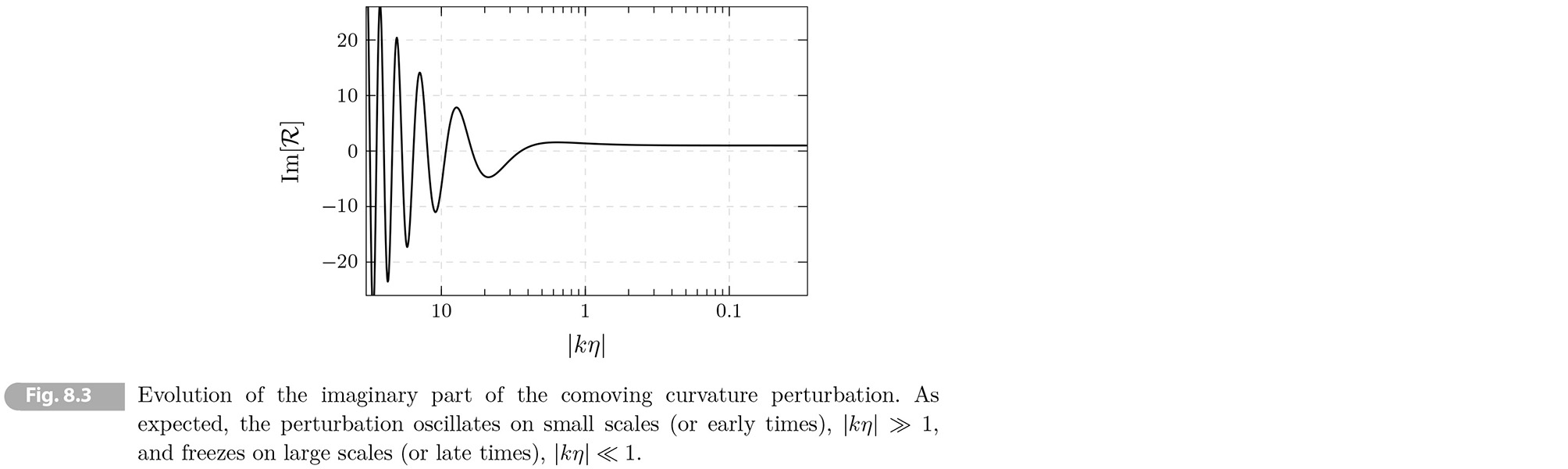
Figure 8.3 shows the evolution of the imaginary part of the comoving curvature perturbation, 𝓡 = 𝑓/𝑧, given the solution (8.64). As expected, the solution oscillates at early times and freezes after horizon crossing. The initial amplitude of the oscillations is set by quantum zero-point fluctuations.
Exercise 8.6 Show that (8.64) implies
(8.65-7) Re[𝓡] = 𝛢[sin(𝑥) - 𝑥 cos(𝑥)], Im[𝓡] = 𝛢[cos(𝑥) + 𝑥 sin(𝑥)], [𝓡] = 𝛢√(1 + 𝑥2),
where 𝑥 ≡ 𝑘𝜂.
[Solution] According to (8.8), since in (8.55) 𝐻 = const and 𝑎 = -(𝐻𝜂)-1,
(a) 𝑧 ≡ 𝑎𝜙̄ʹ/𝓗 = 𝑎√(𝜀/4π𝐺) = -√(𝜀/4π𝐺𝐻2) 1/𝜂.
(b) 𝓡 = 𝑓/𝑧 = -√[(4π𝐺𝐻2)/(2𝜀𝑘3)] 𝑘𝜂 (1 - 𝑖/𝑘𝜂) 𝑒-𝑘𝜂 = √[(4π𝐺𝐻2)/(2𝜀𝑘3)] (𝑖 - 𝑘𝜂) 𝑒-𝑘𝜂 ⇒ 𝓡 = 𝛢(𝑖 - 𝑥) 𝑒-𝑖𝑥
where 𝛢 ≡ √[(4π𝐺𝐻2)/(2𝜀𝑘3)] = const.
(c) Re[𝓡] = 1/2 [𝓡 + 𝓡*] = 𝛢/2[(𝑖 - 𝑥) 𝑒-𝑖𝑥 + (-𝑖 - 𝑥)𝑒𝑖𝑥] = 𝛢 [(𝑒𝑖𝑥 - 𝑒-𝑖𝑥)/2𝑖 - 𝑥 (𝑒𝑖𝑥 + 𝑒-𝑖𝑥)/2] = 𝛢[sin(𝑥) - 𝑥 cos(𝑥)].
(d) Im[𝓡] = 1/2 [𝓡 - 𝓡*] = 𝛢/2𝑖[(𝑖 - 𝑥) 𝑒-𝑖𝑥 - (-𝑖 - 𝑥)𝑒𝑖𝑥] = 𝛢 [(𝑒𝑖𝑥 + 𝑒-𝑖𝑥)/2 + 𝑥 (𝑒𝑖𝑥 - 𝑒-𝑖𝑥)/2𝑖] = 𝛢[cos(𝑥) + 𝑥 sin(𝑥)].
(e) ∣𝓡∣ = √(𝓡*𝓡) = 𝛢√[(-𝑖 - 𝑥)((𝑖 - 𝑥)] = 𝛢√(1 + 𝑥2). ▮
Zero-point fluctuation
Finally, we can predict the quantum statistics of operator
(8.68) 𝑓̂(𝜂, 𝐱) = ∫ d3𝑘/(2π)3 [𝑓𝑘(𝜂)𝑎̂𝐤 + 𝑓𝑘*(𝜂)𝑎̂†-𝐤] 𝑒𝑖𝐤⋅𝐱.
The expectation value of 𝑓̂ vanishes, i.e. ⟨𝑓̂⟩ ≡ ⟨0∣𝑓̂∣0⟩ =0. However, the variance of inflaton fluctuations receives nonzero quantum fluctuations:
(8.69) ⟨∣𝑓̂∣2⟩ ≡ ⟨0∣𝑓̂(𝜂, 𝟬)𝑓̂(𝜂, 𝟬)∣0⟩ = ∫ d3𝑘/(2π)3 ∫ d3𝑘ʹ/(2π)3 ⟨0∣(𝑓𝑘*(𝜂)𝑎̂†-𝐤 + 𝑓𝑘(𝜂)𝑎̂𝐤)(𝑓𝑘ʹ(𝜂)𝑎̂𝐤ʹ + 𝑓𝑘ʹ*(𝜂)𝑎̂†-𝐤ʹ)∣0⟩
= ∫ d3𝑘/(2π)3 ∫ d3𝑘ʹ/(2π)3 𝑓𝑘(𝜂)𝑓𝑘ʹ*(𝜂) ⟨0∣𝑎̂𝐤, 𝑎̂†-𝐤ʹ∣0⟩ = ∫ d3𝑘/(2π)3 ∣𝑓𝑘(𝜂)∣2 = ∫ d ln 𝑘 𝑘3/2π2 ∣𝑓𝑘(𝜂)∣2.
We see that the variance of the quantum fluctuations is determined by the (dimension less) power spectrum of the classical solution:
(8.70) ∆2𝑓(𝑘, 𝜂) ≡ 𝑘3/2π2 ∣𝑓𝑘(𝜂)∣2.
Substituting the Bunch-Davis mode function (8.64) for 𝑓 = 𝑎 𝛿𝜙, we find
(8.71) ∆2𝛿𝜙(𝑘, 𝜂) = ∆𝑓2(𝑘, 𝜂)/𝑎2(𝜂) = (𝐻/2π)2 [1 + (𝑘𝜂)2] 𝑘𝜂→0→ (𝐻/2π)2.
Note that in the superhorizon limit, 𝑘𝜂 → 0, the dimensionless power spectrum ∆𝛿𝜙2 approaches the same constant for all momenta, which is the characteristic of a scale-invariant spectrum.
Although the time dependence of the Hubble rate during inflation is small, it is crucial that it is nonzero. Otherwise, there wouldn't be any evolution and inflation would never end. Moreover, curvature perturbations would be ill-defined since 𝓡 ∝ Ḣ-1 → ∞. To incorporate the effect of a varying 𝐻(𝑡), we evaluate the power spectrum (8.71) at horizon crossing, 𝑘 = 𝑎𝐻, which for each Fourier mode, corresponds to a different moment in time. Since 𝐻 is evolving, this leads to a slight scale dependence of the spectrum
(8.72) ∆2𝛿𝜙(𝑘) ≈ [𝐻(𝑡)/2π]2∣𝑘=𝑎𝐻(𝑡).
Because 𝐻(𝑡) decreases during inflation, the amplitude of fluctuations will be slightly larger for long-wavelength fluctuations which exit the horizon at the beginning of inflation.
From quantum to classical
An important consequence of the stretching of fluctuations from microscopic to macroscopic scales is the fact that the initial quantum fluctuations become classical fluctuations after horizon crossing. To see this, note from (8.64) that the mode function 𝑓𝑘(𝜂) becomes purely imaginary on the superhorizon scales:
(8.73) Re[𝑓𝑘] → 0, [𝑓𝑘] ∝ 𝑎(𝜂).
The field operator and its conjugate momentum then becomes proportional to each other:
(8.74) 𝑓̂𝐤(𝜂) 𝑘𝜂→0→ 𝑓𝑘(𝜂)(𝑎̂𝐤 - 𝑎̂†-𝐤),
(8.75) 𝜋̂𝐤(𝜂) 𝑘𝜂→0→ 𝑓𝑘ʹ(𝜂)(𝑎̂𝐤 - 𝑎̂†-𝐤) ≈ 𝑓𝑘ʹ(𝜂)/𝑓𝑘(𝜂) 𝑓̂𝐤(𝜂).
While both 𝑓̂ ∝ 𝑎(𝜂) and ∆ ∝ 𝑎2(𝜂) grow outside the horizon, the commutator [𝑓̂, 𝜋̂] stays constant. Since the uncertainty ∆𝑓̂∆𝜋̂ is proportional to [𝑓̂, 𝜋̂], a state ∣𝑓𝑘⟩ with a definite field value has an almost definite momentum. Using (8.64), we can compute the ratio
(8.76) 𝑅 ≡ ∆𝑓̂∆𝜋̂/∣𝑓̂∣∣𝜋̂∣ = (ℏ/2)/[ℏ/2 √{1 + (𝑘𝜂)-6}] = 1/√[1 + (𝑘𝜂)-6] 𝑘𝜂→0→ (𝑘𝜂)3 ≪ 1.
We see that the quantum uncertainty is large (𝑅 ~ 1) at early times, but becomes very small (𝑅 ≪ 1) at late times and on large scales.
1 Since the frequency 𝜔𝑘(𝜂) ≡ 𝑘2 - 2/𝜂2 in (8.55) depends only the magnitude 𝑘, the evolution does not depend on direction. The constant operator 𝑎̂𝐤 and 𝑎̂𝐤†, on the other hand, define initial conditions which may depend on direction.
p.s. 한마디로 아주 난해한 chapter입니다! 기초적 내용만을 학습한 양자역학 방정식으로 가득하네요.
몇년 전에 학습한 D. Fleish Schödinger equation (Cambridge University Press, 2020)를 다시 읽고, 추가로,
D. J. Griffiths Introduction to Quantum Mechanics (Pearson Inc. 2nd edition, 2005)를 부분 참조함.
그래도 양자역학의 다양한 용어들의 의미를 대체로 이해할 수 있다는 점에서 큰 위안을 삼음..ㅎ |
|
|