|
김관석
|
2025-01-28 20:37:19, 조회수 : 51 |
- Download #1 : BC_Ab.jpg (229.8 KB), Download : 0

A.3.3 A Mathematical Interlude*
In this section we will fill in some of the mathematical details which is important to get a full appreciation for the logical structure of the theory.
Tensors in general relativity
In SR all physical law must be written in terms of tensors because we want them to be valid in every inertial frame. The same is true in GR, but the theory now deals with non-inertial frame.
Consider a general coordinate transformation 𝑥𝜇 → 𝑥ʹ𝜇(𝑥). The infinitesimal coordinate differentials transform as
(A.83) d𝑥ʹ𝜇 = ∂𝑥ʹ𝜇/∂𝑥𝜈 d𝑥𝜈 ≡ 𝑆𝜇𝜈 d𝑥𝜈,
where the transformation matrix 𝑆𝜇𝜈 play the same role as 𝛬𝜇𝜈 in a Lorentz transformation, but it crucially it now depends on the position 𝑥𝜇. A 4-vector field 𝑉𝜇(𝑥) is an object that transforms in the same way as d𝑥𝜇:
(A.84) 𝑉ʹ𝜇 = 𝑆𝜇𝜈𝑉𝜇.
Note that although d𝑥𝜇 transforms like a vector, 𝑥𝜇 does not.
To determine the transformation of a co-vector 𝑊𝜇, we use that the inner product 𝑊𝜇𝑉𝜇 must be an invariant. The transformation of 𝑊𝜇 therefore involves the inverse matrix
(A.85) 𝑊ʹ𝜇 = (𝑆-1)𝜇𝜈 = ∂𝑥𝜈/∂𝑥ʹ𝜇 𝑊𝜈.
By inspection of (A.84) and (A.85) we can guess that an arbitrary tensor transform as
(A.86) (𝛵ʹ)𝜇1∙ ∙ ∙ 𝜇𝑚𝜈1∙ ∙ ∙ 𝜈𝑛 = 𝑆𝜇1𝜎1 ∙ ∙ ∙ (𝑆-1)𝜈1𝜌1 ∙ ∙ ∙ 𝛵𝜎1∙ ∙ ∙ 𝜎𝑚𝜎1∙ ∙ ∙ 𝜎𝑛.
This is the generalization of the analogous result (A.16) in SR. An important tensor is the metric tensor 𝑔𝜇𝜈. Its transformation can also be derived from the invariance of the line element:
(A.87) d𝑠2 = 𝑔ʹ𝜇𝜈(𝑥ʹ)d𝑥ʹ𝜇d𝑥ʹ𝜈 = 𝑔𝜌𝜎(𝑥)d𝑥𝜌d𝑥𝜎 = 𝑔𝜌𝜎(𝑥) ∂𝑥𝜌/∂𝑥ʹ𝜇 ∂𝑥𝜎/∂𝑥ʹ𝜈 d𝑥ʹ𝜇d𝑥ʹ𝜈,
so that
(A.88) 𝑔ʹ𝜇𝜈 = 𝑔𝜌𝜎 ∂𝑥𝜌/∂𝑥ʹ𝜇 d𝑥𝜎/d𝑥ʹ𝜈 ≡ (𝑆-1)𝜇𝜌(𝑆-1)𝜈𝜎𝑔𝜌𝜎,
which is consistent with the general transformation law (A.86).
Derivatives of tensors
Let us see how derivatives of scalars, vectors, and tensors transform under a general coordinate transformation. Consider first the partial derivative of a scalar field, ∂𝜇𝜙. Since 𝜙ʹ(𝑥ʹ) = 𝜙(𝑥), we get
(A.89) ∂𝜇𝜙ʹ(𝑥ʹ) = ∂𝜙ʹ(𝑥ʹ)/d𝑥ʹ𝜇 = ∂𝑥𝜈/∂𝑥ʹ𝜇 ∂𝜙(𝑥)/d𝑥𝜈 ≡ (𝑆-1)𝜇𝜈 ∂𝜈𝜙(𝑥).
Unsurprisingly, ∂𝜇𝜙 transforms like a covariant vector. However, when we take the partial derivative of a vector, ∂𝜆𝑉𝜇, this case is different:
(A.90) ∂ʹ𝜆𝑉ʹ𝜇(𝑥ʹ) = ∂𝑉ʹ𝜇(𝑥ʹ)/∂𝑥ʹ𝜆 = ∂𝑥𝜎/∂𝑥ʹ𝜆 ∂/∂𝑥𝜎 [𝑆𝜇𝜈(𝑥)𝑉𝜈(𝑥)]
(A.91) = (𝑆-1)𝜆𝜎𝑆𝜇𝜈∂𝜎𝑉𝜈 + [(𝑆-1)𝜆𝜎∂𝜎𝑆𝜇𝜈]𝑉𝜈.
The second term in (A.91) spoils the transformation law. So we would like to define a new derivative ∇𝜆𝑉𝜇 that does transform like a tensor:
(A.92) ∇ʹ𝜆𝑉ʹ𝜇 = (𝑆-1)𝜆𝜎𝑆𝜇𝜈∇𝜎𝑉𝜈.
In the next exercise we will show that the covariant derivative defined in (A. 72) has precisely this property.4
Exercise A.3 Show that the Christoffel symbol defined in (A.63) transform as
(A.93) 𝛤ʹ𝜇𝜆𝜈 = ∂𝑥ʹ𝜇/∂𝑥𝜌 ∂𝑥𝜎/∂𝑥ʹ𝜆 ∂𝑥𝜂/∂𝑥ʹ𝜈 𝛤𝜌𝜎𝜂 + ∂𝑥ʹ𝜇/∂𝑥𝜂 ∂2𝑥𝜂/∂𝑥ʹ𝜆∂𝑥ʹ𝜈 = 𝑆𝜇𝜌(𝑆-1)𝜆𝜎(𝑆-1)𝜈𝜂 𝛤𝜌𝜎𝜂 + 𝑆𝜇𝜂(𝑆-1)𝜆𝜌∂𝜌(𝑆-1)𝜈𝜂.
We see that the Christoffel symbol does not transform as a tensor. Show that (A.92) holds!
Hint: We need ∂𝑆-1 = -𝑆-1(∂𝑆)𝑆-1, which holds because 𝑆𝑆-1 = 1. [Solution is omitted.]
So far, we only saw the covariant derivative of a contravariant vector:
(A.94) ∇𝜇𝑉𝜈 = ∂𝜇𝑉𝜈 + 𝛤𝜈𝜇𝛼𝑉𝛼.
To determine the covariant derivative of a covariant vector consider how it acts on the scalar 𝑓 ≡ 𝑊𝜈𝑉𝜈. Using ∇𝜇𝑓 = ∂𝜇𝑓, we get
(A.95) ∇𝜇𝑊𝜈 = ∂𝜇𝑊𝜈 - 𝛤𝛼𝜇𝜈𝑊𝛼.
Exercise A.4 Derive (A.95) from (A.94)
[Solution] Using ∇𝜇𝑓 = ∂𝜇𝑓, we find
(a) ∇𝜇(𝑊𝜈𝑉𝜈) = ∂𝜇(𝑊𝜈𝑉𝜈) = (∂𝜇𝑊𝜈)𝑉𝜈 + 𝑊𝜈(∂𝜇𝑉𝜈)
(b) ∇𝜇(𝑊𝜈𝑉𝜈) = (∇𝜇𝑊𝜈)𝑉𝜈 + 𝑊𝜈(∇𝜇𝑉𝜈) = (∇𝜇𝑊𝜈)𝑉𝜈 + 𝑊𝜈(∂𝜇𝑉𝜈 + 𝛤𝜈𝜇𝛼𝑉𝛼).
Comparing the last equality in (a) and (b), we find
(c) (∂𝜇𝑊𝜈)𝑉𝜈 + 𝑊𝜈(∂𝜇𝑉𝜈) = (∇𝜇𝑊𝜈)𝑉𝜈 + 𝑊𝜈(∂𝜇𝑉𝜈 + 𝛤𝜈𝜇𝛼𝑉𝛼) ⇒ (∇𝜇𝑊𝜈)𝑉𝜈 = (∂𝜇𝑊𝜈)𝑉𝜈 - 𝛤𝜈𝜇𝛼𝑊𝜈𝑉𝛼 = (∂𝜇𝑊𝜈 - 𝛤𝛼𝜇𝜈𝑊𝛼)𝑉𝜈 ⇒
(d) ∇𝜇𝑊𝜈 = ∂𝜇𝑊𝜈 - 𝛤𝛼𝜇𝜈𝑊𝛼. ▮
The covariant derivative of the mixed tensor 𝛵𝜇𝜈 can be derive similarly by considering 𝑓 ≡ 𝛵𝜇𝜈𝑉𝜈𝑊𝜇. This gives
(A.96) ∇𝜎𝛵𝜇𝜈 = ∂𝜎𝛵𝜇𝜈 + 𝛤𝜇𝜎𝛼𝛵𝛼𝜈 - 𝛤𝛼𝜎𝜈𝛵𝜇𝛼.
From flat to curved spacetime
As we saw the covariant derivative of a tensor transforms like a tensor, while the partial derivative does not, A simple prescription to upgrade equations from flat space to curved space is to replace every partial derivative by a covariant derivative, ∂𝜇 → ∇𝜇.5 In (A.20) we showed that the inhomogeneous Maxwell equations can be written as ∂𝜈𝐹𝜇𝜈 = 𝐽𝜇. The generalization of this equation to curved spacetime is simply
(A.97) ∇𝜈𝐹𝜇𝜈 = 𝐽𝜇,
where the dependence on the metric is encoded and this describes the dynamics of electromagnetic fields in GR. Similarly, we saw that the conservation of the energy-momentum tensor in SR implies ∂𝜈𝛵𝜇𝜈 = 0. In GR this becomes
(A.98) ∇𝜈𝛵𝜇𝜈 = 0.
The covariant derivative depends on the metric and hence defines a coupling between matter and the gravitational degrees of freedom.
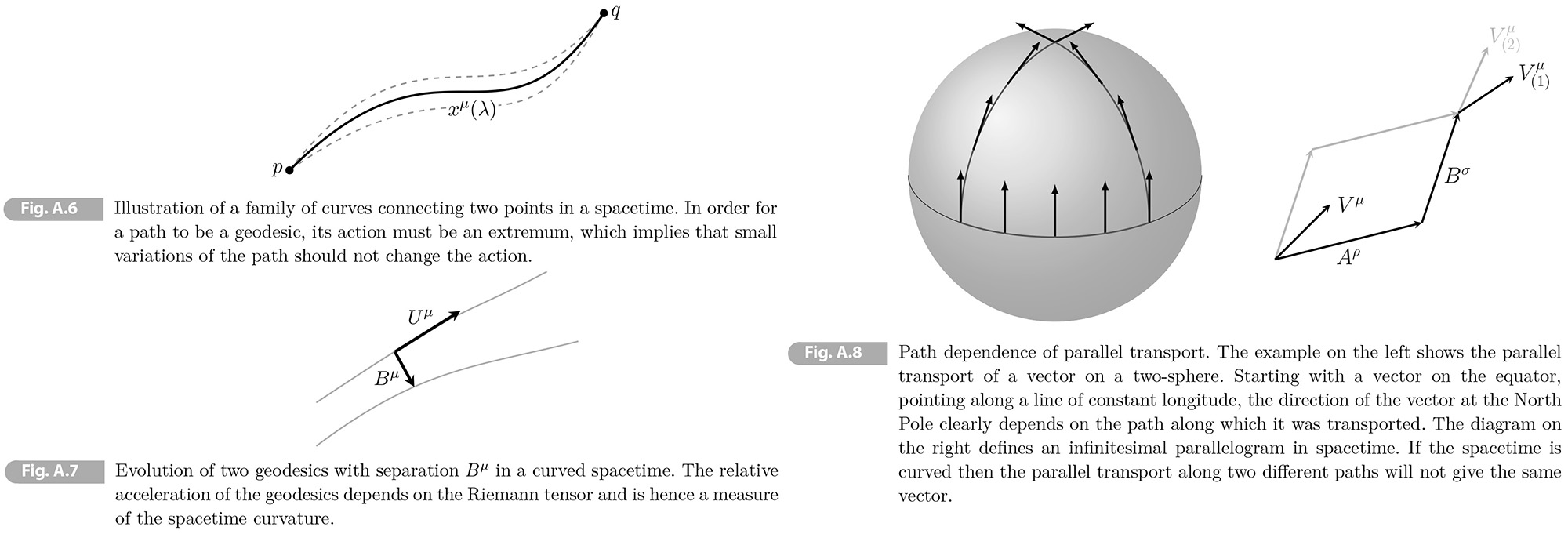
Parallel transport and geodesics
Given the notion of a covariant derivative, we can define the concept of a parallel transport of a tensor. In flat spacetime "parallel transport" simply means translating a vector along a curve while "keeping it constant." So a vector 𝑉𝜇 is constant along a curve 𝑥𝜇(𝜆) if its components don't depend on the parameter 𝜆:
(A.99) d𝑉𝜇/d𝜆 = d𝑥𝜈/d𝜆 ∂𝜈𝑉𝜇 = 0. (flat spacetime).
We generalize this to curved spacetimes by replacing the partial derivative in (A.99) by a covariant derivative. This gives so-called directional covariant derivative. a vector is parallel transport in GR if the directional covariant derivative of the vector along a curve vanishes:
(A.100) 𝐷𝑉𝜇/𝐷𝜆 = d𝑥𝜈/d𝜆 ∇𝜈𝑉𝜇 = 0. (curved spacetime).
Although we wrote the equation for a vector field, an analogous equation applies for arbitrary tensors. Write out te covariant derivative, the equation of parallel transport becomes
(A.101) d𝑉𝜇/d𝜆 + 𝛤𝜇𝜎𝜈 d𝑥𝜎/d𝜆 𝑉𝜇 = 0,
which tells us that the components of the vector will now change along the curve and that this change is determined by the connection 𝛤𝜇𝜎𝜈.
Using parallel transport, we can give an alternative definition of a geodesic as the curve generated by a tangent vector d𝑥𝜇/d𝜆 that is transported parallel to itself. This generalizes the notion of a straight line in flat space, which can be thought of as the path that parallel transports its own tangent vector. Substituting 𝑉𝜇 = d𝑥𝜇/d𝜆 into (A.101), we get
(A.102) d2𝑥𝜇/d𝜆2 + 𝛤𝜇𝜎𝜈 d𝑥𝜎/d𝜆 d𝑥𝜈/d𝜆 = 0,
which is indeed the same as the geodesic equation, if we write 𝜆 = 𝑎𝑥 + 𝑏 for a massive particle.
A.4 The Einstein Equation
So far. we described how test particles move in arbitrary curved spacetime. Next we will discuss the spacetime curvature is determined by the local matter distribution. We are in search of the following relationship:
(A.103) (a measure of local spacetime curvature) = (a measure of local stress-energy density).
A.4.1 Tidal Forces and Curvature
We will study the relative acceleration of two test particles in GR and find that the motion is determined by the Riemann tensor an object of fundamental importance in differential geometry.
Consider two particles 𝐱(𝑡) and 𝐱(𝑡) + 𝐛(𝑡). In Newtonian gravity they satisfy
(A.104-5) d2𝑥𝑖/d𝑡2 = -∂𝑗𝛷(𝑥𝑗), d2(𝑥𝑖 + 𝑏𝑖)/d𝑡2 = -∂𝑗𝛷(𝑥𝑗 + 𝑏𝑗)
Subtracting (A.104) from (A.105), and expanding the result to first order, we get
(A.106) d2𝑏𝑖/d𝑡2 = -∂𝑗∂𝑖𝛷 𝑏𝑗. [verification needed]
We see the relativistic acceleration of particles is determines by the tidal tensor ∂𝑖∂𝑗𝛷. The Poisson equation relates the trace of this tidal tensor to the mass density
(A.107) ∇2𝛷 = ∂𝑖∂𝑗𝛷 = 4π𝐺𝜌.
Let us find of (A.106) in GR where it is called the geodesic deviation equation. The analog of the tidal tensor will give us local measure of the spacetime curvature. Its trace will lead to the Einstein equation.
Consider two geodesics separated by an infinitesimal vector 𝛣𝜇 (see Fig. A.7). We define the "relative velocity" of the two geodesics as the directional covariant derivative of 𝛣𝜇 along one of the geodesics:
(A.108) 𝑉𝜇 ≡ 𝐷𝛣𝜇/𝐷𝜏 = 𝑈𝜈∇𝜈𝛣𝜇 = d𝛣𝜇/d𝜏 + 𝛤𝜇𝜎𝜈𝛣𝜎, where 𝑈𝜇 = d𝑥/d𝜏.
The "relative acceleration" is
(A.109) 𝛢𝜇 ≡ 𝐷2𝛣𝜇/𝐷𝜏2 = 𝑈𝜈∇𝜈𝑉𝜇 = d𝑉𝜇/d𝜏 + 𝛤𝜇𝜎𝜈𝑉𝜎.
After some work (see below the derivation), we find
(A.110) 𝐷2𝛣𝜇/𝐷𝜏2 = -𝑅𝜇𝜈𝜎𝜌𝑈𝜈𝑈𝜎𝛣𝜌.
where we defined the Riemann tensor
(A.111) 𝑅𝜇𝜈𝜎𝜌 ≡ ∂𝜌𝛤𝜇𝜈𝜎 - ∂𝜎𝛤𝜇𝜈𝜌 + 𝛤𝜇𝜌𝜆𝛤𝜆𝜈𝜎 - 𝛤𝜇𝜎𝜆𝛤𝜆𝜈𝜌.
This scary beast is the analog of the tidal tensor in Newtonian gravity.
Derivation Substituting (A.108) into (A.109), we get
(A.112) 𝛢𝛼 = d𝑉𝛼/d𝜏 + 𝛤𝛼𝛽𝛾𝑈𝛽𝑉𝛾 = d/d𝜏 (d𝛣𝛼/d𝜏 + 𝛤𝛼𝛽𝛾𝑈𝛽𝛣𝛾) + 𝛤𝛼𝛽𝛾𝑈𝛽 (d𝛣𝛾/d𝜏 + 𝛤𝛾𝛿𝜖𝑈𝛿𝛣𝜖)
= d2𝛣𝛾/d𝜏2 + d𝛤𝛼𝛽𝛾/d𝜏 𝑈𝛽𝛣𝛾 + 𝛤𝛼𝛽𝛾 d𝑈𝛽/d𝜏 + 2𝛤𝛼𝛽𝛾𝑈𝛽 d𝑈𝛽/d𝜏 + 𝛤𝛼𝛽𝛾𝛤𝛾𝛿𝜖𝑈𝛽𝑈𝛿𝛣𝜖.
(A.113-4) d𝛤𝛼𝛽𝛾/d𝜏 = -𝑈𝛿∂𝛿𝛤𝛼𝛽𝛾, d𝑈𝛽/d𝜏 = -𝛤𝛽𝛿𝜖𝑈𝛿𝑈𝜖),
where (A.114) follows fr the geodesic equation (A.71). We therefore get
(A.115) 𝛢𝛼 = d2𝛣𝛾/d𝜏2 + 2𝛤𝛼𝛽𝛾𝑈𝛽 d𝑈𝛽/d𝜏 + (∂𝛿𝛤𝛼𝛽𝛾 - 𝛤𝜖𝛿𝛽𝛤𝛼𝜖𝛾 + 𝛤𝛼𝛽𝜖𝛤𝜖𝛿𝛾) 𝑈𝛽𝑈𝛿𝛣𝛾,
where we relabeled some dummy indices to extract 𝑈𝛽𝑈𝛿𝛣𝛾 from three of terms. To replace the derivatives of 𝛣𝛼, we note that 𝑥𝛼(𝜏) + 𝛣𝛼(𝜏) obeys the geodesic equation
(A.116) d2(𝑥𝛼 + 𝛣𝛼)𝛾/d𝜏2 + 𝛤𝛼𝛽𝛾(𝑥𝛿 + 𝛣𝛿) d(𝑥𝛽 + 𝛣𝛽)/d𝜏 d(𝑥𝛾 + 𝛣𝛾)/d𝜏 = 0.
Subtracting the geodesic equation for 𝑥𝛼(𝜏) and expanding the result to linear order in 𝛣𝛼, we get
(A.117) d2𝛣𝛾/d𝜏2 + 2𝛤𝛼𝛽𝛾𝑈𝛽 d𝑈𝛽/d𝜏 = -∂𝛿𝛤𝛼𝛽𝛾𝛣𝛿𝑈𝛽𝑈𝛾 = -∂𝛾𝛤𝛼𝛽𝛿𝑈𝛽𝑈𝛿𝛣𝛾,
Substituting this into (A.115), we find
(A.118) 𝛢𝛼 = -(∂𝛾𝛤𝛼𝛽𝛿 - ∂𝛿𝛤𝛼𝛽𝛾 + 𝛤𝜖𝛿𝛽𝛤𝛼𝜖𝛾 - 𝛤𝛼𝛽𝜖𝛤𝜖𝛿𝛾)≡ 𝑅𝛼𝛽𝛾𝛿 𝑈𝛽𝑈𝛿𝛣𝛾. ▮
In the local inertial frame of a freely falling observer, with 4-velocity 𝑈𝜇 = (1, 0, 0, 0), the geodesic deviation equation becomes
(A.119) d2𝛣𝜇/d𝜏2 = -𝑅𝜇0𝜈0𝛣𝜈.
For the static, weak-field metric (A.54), we have 𝑅𝑖0𝑗0 = ∂𝑗𝛤𝑖00 = ∂𝑖𝑗𝛷 and (A.119) reduces to Newtonian result (A.106). [RE (A.74-81)]
A.4.2 The Mathematics of Curvature*
There is a lot of beautiful mathematics underlying the physics of spacetime curvature. We will see a very brief snapshot though.
Parallel transport and curvature
An important property of the parallel transport of a vector on a curved manifold is that it depends on the path along which the vector is transported. This is illustrated in Fog. A.8 for the case 2-sphere.
This path dependence of the parallel transport gives another way diagnose whether the spacetime is curved. Consider a parallelogram spanned by the infinitesimal vectors 𝛢𝜌 and 𝛣𝜎 (see Fig. A.8) and imagine parallel transporting a vector 𝑉𝜇. From the equation of parallel transport (A.101), we have that the change of the vector along a side 𝛿𝑥𝜌 is
(A.120) 𝛿𝑉𝜇 = -𝛤𝜇𝜈𝜌𝑉𝜈𝛿𝑥𝜌.
On "path 1" we parallel transport the vector first along 𝛢𝜌 and then along 𝛣𝜎 while on "path 2" we reverse the order (giving the gray path in Fig. A.8). Using (A.120), we get
(A.121) 𝛿𝑉𝜇(1) = -𝛤𝜇𝜈𝜌(𝑥)𝑉𝜈(𝑥)𝛢𝜌 - 𝛤𝜇𝜈𝜌(𝑥 + 𝛢)𝑉𝜈(𝑥 + 𝛢) 𝛣𝜌, 𝛿𝑉𝜇(2) = -𝛤𝜇𝜈𝜌(𝑥)𝑉𝜈(𝑥)𝛣𝜌 - 𝛤𝜇𝜈𝜌(𝑥 + 𝛣)𝑉𝜈(𝑥 + 𝛣) 𝛢𝜌,
and the difference is
(A.122) 𝛿𝑉𝜇 ≡ 𝛿𝑉𝜇(1) - 𝛿𝑉𝜇(2) = ∂𝜎(𝛤𝜇𝜈𝜌𝑉𝜈) 𝛣𝜎𝛢𝜌 - ∂𝜎(𝛤𝜇𝜈𝜌𝑉𝜈) 𝛢𝜎𝛣𝜌,
where we have Taylor expanded the arguments for small 𝛢𝜌 and 𝛣𝜌. Swapping the dummy indices on he second term, 𝜌 ⟷ 𝜎, and differentiating the products, we find
(A.123) 𝛿𝑉𝜇 = (∂𝜎𝛤𝜇𝜈𝜌𝑉𝜈 + 𝛤𝜇𝜈𝜌∂𝜎𝑉𝜈 - ∂𝜌𝛤𝜇𝜈𝜌𝑉𝜈 + 𝛤𝜇𝜈𝜌∂𝜌𝑉𝜈)𝛢𝜌𝛣𝜎.
Using (A.101) again, we have ∂𝜎𝑉𝜈 = -𝛤𝜈𝜎𝜆𝑉𝜆 and hence (A.123) becomes
(A.124) 𝛿𝑉𝜇 = 𝑅𝜇𝜈𝜌𝜎𝑉𝜈𝛢𝜌𝛣𝜎,
where 𝑅𝜇𝜈𝜌𝜎 is the Riemann tensor as defined in (A.111)
Properties of the Riemann tensor
Only 20 of the 44 = 256 components of 𝑅𝜇𝜈𝜌𝜎 are independent, because the Riemann tensor has a lot of symmetries that relate its different components. These symmetries are easiest present to present for the the Riemann tensor with only lower indices 𝑅𝜇𝜈𝜌𝜎 = 𝑔𝜇𝜆𝑅𝜆𝜈𝜌𝜎. We then have
(A.125-8) 𝑅𝜇𝜈𝜌𝜎 = -𝑅𝜈𝜇𝜌𝜎, 𝑅𝜇𝜈𝜌𝜎 = -𝑅𝜇𝜈𝜎𝜌, 𝑅𝜇𝜈𝜌𝜎 = 𝑅𝜌𝜎𝜇𝜈, 𝑅𝜇𝜈𝜌𝜎 + 𝑅𝜇𝜌𝜎𝜈 + 𝑅𝜇𝜎𝜈𝜌 = 0.
In addition, the Riemann tensor satisfies an important differential identity called the Bianchi identity, states that the sum of the cyclic permutations of the first three indices of ∇𝜆𝑅𝜇𝜈𝜌𝜎 vanishes:
(A.129) ∇𝜆𝑅𝜇𝜈𝜌𝜎 + ∇𝜈𝑅𝜆𝜇𝜌𝜎 + ∇𝜇𝑅𝜆𝜈𝜌𝜎 = 0.
This is the analog of homogeneous Maxwell equation ∂𝜆𝐹𝜇𝜈 + ∂𝜈𝐹𝜆𝜇 + ∂𝜇𝐹𝜈𝜆 = 0.
A.4.3 Guessing the Einstein Equation
First, we will "guess" it. Then, we will construct an action for the metric and show that the corresponding equation of motion lead to the same Einstein equation.
We are searching for the relativistic generalization of the Poission equation:
(A.130) ∇2𝛷 = 4π𝐺𝜌.
We would like to write this equation in tensorial form, so that it is valid independently of the choice of coordinates. On the right side 𝜌 suggests that 𝛵𝜇𝜈 should appear, while on the left side 𝛷 suggests that we expect an object with two derivatives acting on the metric. We recall that the Poisson equation is the trace of the tidal tensor, ∂𝑖∂𝑗𝛷, and the generalization of the tidal tensor is the Riemann tensor, 𝑅𝜇𝜈𝜌𝜎. This suggests that the trace of the Riemann tensor would be an interesting object. Taking the trace means contracting the upper index with a lower index and so this leads to the Ricci tensor
(A.131) 𝑅𝜇𝜈 ≡ 𝑅𝜆𝜇𝜆𝜈 = ∂𝜆𝛤𝜆𝜇𝜈 - ∂𝜈𝛤𝜆𝜇𝜆 + 𝛤𝜆𝜌𝜆𝛤𝜌𝜇𝜈 - 𝛤𝜌𝜇𝜆𝛤𝜆𝜈𝜌.
This gas all the properties we want: it is a symmetric (0, 2) tensor with second-order derivatives acting on the metric.
A first and second guess
Einstein's first guess for the field equation of GR was
(A.132) 𝑅𝜇𝜈 =? 𝜅𝛵𝜇𝜈, where 𝜅 is a constant.
However, it doesn't work because we can have ∇𝜇𝑅𝜇𝜈 ≠ 0, which would be inconsistent with the conservation of energy-momentum tensor, ∇𝜇𝛵𝜇𝜈 = 0. To see this, we consider the double contraction of the Bianchi identity (A. 129):
(A.133) 0 = 𝑔𝜎𝜆𝑔𝜇𝜌(∇𝜆𝑅𝜇𝜈𝜌𝜎 + ∇𝜈𝑅𝜆𝜇𝜌𝜎 + ∇𝜇𝑅𝜆𝜈𝜌𝜎) = ∇𝜎𝑅𝜈𝜎 - ∇𝜈𝑅 + ∇𝜇𝑅𝜈𝜌,
where 𝑅 = 𝑔𝜇𝜈 is the Ricci scalar. This implies that
(A.134) ∇𝜇𝑅𝜇𝜈 = 1/2 ∇𝜈𝑅,
which doesn't vanish except where 𝑅 (and hence 𝛵 = 𝑔𝜇𝜈𝛵𝜇𝜈) is a constant.
To fix the problem we simply not that (A. 134) can be written as
(A.135) ∇𝜇(𝑅𝜇𝜈 - 1/2 𝑔𝜇𝜈𝑅) = 0.
This suggests an alternative measure of curvature, the so called Eisenstein tensor.
(A.136) 𝐺𝜇𝜈 ≡ 𝑅𝜇𝜈 - 1/2 𝑔𝜇𝜈𝑅.
which is consistent with the conservation of the energy-momentum tensor. So the improved guess of the Einstein equation is
(A.137) 𝐺𝜇𝜈 =? 𝜅𝛵𝜇𝜈.
Now, we have to verify that it reduces to the Poisson equation (A. 136) in the Newtonian limit.
Newtonian limit
Contracting both sides of (A.137) gives
(A.138) 𝑅 = -𝜅𝛵, [verification needed]
where we use that 𝛿𝜇𝜇 = 4. Substituting this back into (A.137), we get trace-reverced Einstein equation:
(A.139) 𝑅𝜇𝜈 = 𝜅(𝛵𝜇𝜈 - 1/2 𝑔𝜇𝜈𝛵).
In the Newtonian limit, the energy-momentum tensor takes the form of a pressureless fluid, with 𝛵00 = 𝜌 and 𝑔00𝛵00 ≈ -𝛵00 = -𝜌. Note that we have taken 𝜌 to be small and could used the unperturbated metric at leading order. The temporal component of (A.139) is
(A.140) 𝑅00 = 1/2 𝜅𝜌.
We would like to evaluate 𝑅00 in the static, weak-field limit, where the metric can be written as 𝑔𝜇𝜈 = 𝜂𝜇𝜈 + 𝘩𝜇𝜈, cf. (A.77). In addition
(A.141) 𝑅00 = 𝑅𝑖0𝑖0 = ∂𝑖𝛤𝑖00 - ∂0𝛤𝑖𝑖0 + 𝛤𝑖𝑗𝜆𝛤𝜆00 - 𝛤𝑖0𝜆𝛤𝜆𝑗0 = ∂𝑖𝛤𝑖00.
Where we used 𝑅0000 = 0 and dropped the terms of the form 𝛤2 which are second order in the metric perturbation, because the the Christoffel symbols are first order.[verification needed] We also dropped ∂0𝛤𝑖𝑖0 because the metric perturbation is assumed to be time independent. In (A.78) we have 𝛤𝑖00 = -1/2 ∂𝑖𝘩00. At first order in the metric perturbation, we find
(A.142) 𝑅00 = 1/2 ∇2𝘩00,
and (A.140) becomes
(A.143) ∇2𝘩00 = -𝜅𝜌.
Recall 𝘩00 = -2𝛷 in (A.140) reproduce the Poisson equation (A.130) if 𝜅 = 8𝜋𝐺.
The Einstein equation
The final form of the Einstein equation then is
(A.144) 𝐺𝜇𝜈 = 8π𝐺 𝛵𝜇𝜈.
This is one of the most beautiful equations ever written down. It describes a wide range of phenomena from Newtonian physics to the expansion of the universe and black holes.
Note that (A.144) are ten second-order partial differential equations for the metric. Because the Bianchi identity, ∇𝜇𝐺𝜇𝜈 = 0, imposes four constraints, we have only six independent equations.
This counting makes sense since there are four coordinate transformations and hence the metric has six independent components.
A.4.4 Einstein-Hilbert Action
An alternative way of deriving the Einstein equations from an action principle. The action must be an integral over a scalar function. Moreover, this scalar function should be a measure of the local spacetime curvature and be at most second order in derivatives of the metric. The unique such object is Ricci scalar8 and the corresponding Einstein-Hilbert action is
(A.145) 𝑆 = ∫ d4𝑥√(-𝑔) 𝑅,
where 𝑔 ≡ det 𝑔𝜇𝜈 is the determinant of the metric. The factor of √(-𝑔) was introduced so that the volume element d4𝑥√(-𝑔) is invariant under a coordinate transformation.
The Einstein equation follows by varying the action with respect to the (inverse) metric. Writing the Ricci scalar as 𝑅 = 𝑔𝜇𝜈𝑅𝜇𝜈, we have
(A.146) 𝛿𝑆 = ∫ d4𝑥 [𝛿√(-𝑔) 𝑔𝜇𝜈𝑅𝜇𝜈 + √(-𝑔) 𝛿𝑔𝜇𝜈 𝑅𝜇𝜈 + √(-𝑔) 𝑔𝜇𝜈 𝛿𝑅𝜇𝜈].
It can be shown that the last term is a total derivative 𝑔𝜇𝜈 𝛿𝑅𝜇𝜈 = ∇𝜇𝑋𝜇, with 𝑋𝜇 ≡ 𝑔𝜌𝜈 𝛿𝛤𝜇𝜌𝜈 - 𝑔𝜇𝜈 𝛿𝛤𝜌𝜈𝜌, and can be dropped withot affecting the equation of motion. Te evaluate the first term, we use that
(A.147) 𝛿√(-𝑔) = -1/2 √(-𝑔) 𝑔𝜇𝜈 𝛿𝑔𝜇𝜈.
To prove this idensity, we have to use that any diagonalizable matrix 𝑀 satisfies log(det 𝑀) = Tr(log 𝑀). Substituting (A.147) into (A.146), we find
(A.148) 𝛿𝑆 = ∫ d4𝑥 (𝑅𝜇𝜈 - 1/2 𝑔𝜇𝜈𝑅) 𝛿𝑔𝜇𝜈.
For the action to be an extremum, this variation must vanish for arbitrary 𝛿𝑔𝜇𝜈. This is only case if 𝐺𝜇𝜈 = 0, which is the vacuum Einstein equation.
Exercise A.5 Show that the last term in (A.146) is a total derivative
(A.149) 𝑔𝜇𝜈 𝛿𝑅𝜇𝜈 = ∇𝜇𝑋𝜇, with 𝑋𝜇 ≡ 𝑔𝜌𝜈 𝛿𝛤𝜇𝜌𝜈 - 𝑔𝜇𝜈 𝛿𝛤𝜌𝜈𝜌.
Hint: We may use that 𝛤𝜇𝜌𝜈 is a tensor, although 𝛤𝜇𝜌𝜈 is not. Consider "normal coordinates" at a point 𝑝, for which 𝛤𝜇𝜌𝜈(𝑝) = 0. Compute 𝛿𝑅𝜇𝜈 in these coordinates. The result is a tensor equation and therefore holds in all coordinate systems.
[Solution] If we choose to work in normal coordinates 𝛤𝜇𝜌𝜈(𝑝) = 0, we have
(a) 𝛿𝑅𝜇𝜈 = ∂𝜆𝛿𝛤𝜆𝜇𝜈 - ∂𝜈𝛿𝛤𝜆𝜇𝜆 + 𝛤𝜆𝜌𝜆𝛤𝜌𝜇𝜈 - 𝛤𝜌𝜇𝜆𝛤𝜆𝜈𝜌 = ∇𝜆𝛿𝛤𝜆𝜇𝜈 - ∇𝜈𝛿𝛤𝜆𝜇𝜆
So we find
(b) 𝑔𝜇𝜈 𝛿𝑅𝜇𝜈 = 𝑔𝜇𝜈 (∇𝜎𝛿𝛤𝜎𝜇𝜈 - ∇𝜈𝛿𝛤𝜎𝜇𝜎) = ∇𝜎 (𝑔𝜇𝜈𝛿𝛤𝜎𝜇𝜈) - ∇𝜈 (𝑔𝜇𝜈𝛿𝛤𝜎𝜇𝜎) = ∇𝜎 (𝑔𝜇𝜈𝛿𝛤𝜎𝜇𝜈 - 𝑔𝜇𝜎𝛿𝛤𝜌𝜇𝜌) = ∇𝜎𝑋𝜎. ▮
A.4.5 Including Matter
To get the non-vacuum Einstein equation, we add an action for matter to Einstein-Hilbert action. The complete action is
(A.150) 𝑆 = 1/2𝜅 ∫ d4𝑥√(-𝑔) 𝑅 + 𝑆𝑀,
where the constant 𝜅 allows for a difference in the relative normalization of the gravitational action and the matter action. Varying this action with respect to the metric gives
(A.151) 𝑆 = 1/2 ∫ d4𝑥√(-𝑔) (1/𝜅 𝐺𝜇𝜈 - 𝛵𝜇𝜈) 𝛿𝑔𝜇𝜈,
where we defined the energy-momentum tensor as
(A.152) 𝛵𝜇𝜈 ≡ -2/√(-𝑔) 𝛿𝑆𝑀/𝛿𝑔𝜇𝜈. The action (A.150) has an extremum when the metric satisfies (A.137): 𝐺𝜇𝜈 = 𝜅𝛵𝜇𝜈. Fixing the constant 𝜅 in the same way before gives the Einstein equation (A.144).
A.4.6 The Cosmological Constant
There is one other term that can be added to the left side of the Einstein equation which is consistent with the local conservation of 𝛵𝜇𝜈, namely a term of the form 𝛬𝑔𝜇𝜈 = 0. Einstein added such a term and called it the cosmological constant. The modified form of the Einstein equation is
(A.153) 𝐺𝜇𝜈 + 𝛬𝑔𝜇𝜈 = 8π𝐺 𝛵𝜇𝜈.
It has also become common practice to identify this cosmological constant with the stress-energy of the vacuum (if any) and include it on the right side as a contribution to the energy-momentum tensor. The action leading to (A.153) is
(A.154) 𝑆 = 1/16π𝐺 ∫ d4𝑥√(-𝑔) (𝑅 - 2𝛬) + 𝑆𝑀.
We see that the cosmological constant corresponds to a pure volume term in the action.
A.4.7 Some Simple Solutions
The Einstein equations are complicated nonlinear functions of the metric, but a few exact solutions exist in solution with a large amount of symmetry. We will first consider the vacuum Einstein equation (𝛵𝜇𝜈 = 0) with a cosmological constant. Contracting both sides of (A. 153) with the metric, we get 𝑅 = 4𝛬 and hence
(A.155) 𝑅𝜇𝜈 = 𝛬𝑔𝜇𝜈.
There are a few famous solutions to this equation:
• First, we set 𝛬 = 0. The Minkowski line elements,
(A.156) d𝑠2 = -d𝑡2 + d𝐱2,
satiafies the vacuum Einstein equation 𝑅𝜇𝜈 = 0. A more nontrivial solution to the same equation is the Schwarzschild metric:
(A.157) d𝑠2 = -(1 - 2𝐺𝑀/𝑟) d𝑡2 + (1 - 2𝐺𝑀/𝑟)-1 d𝑟2 + 𝑟2d𝛺22,
where d𝛺22 ≡ d𝜃2 + sin2𝜃 d𝜙2 is the metric on the unit 2-sphere. This solution describes the spacetime around a spherically symmetric object of mass 𝑀.
• Next, we consider the case of positive cosmological constant, 𝛬 > 0. The corresponding solution to the Einstein equation is de Sitter space (in static patch coordinates):
(A.158) d𝑠2 = -(1 - 𝑟2/𝑅2) d𝑡2 + (1 - 𝑟2/𝑅2)-1 d𝑟2 + 𝑟2d𝛺22,
where 𝑅2 ≡ 3/𝛬. The static patch coordinates cover only part of the de Sitter geometry, namely that accessible to a single observer which is bounded by the cosmological horizon at 𝑟 = 𝑅. Alternative coordinates that cover the whole space are so-called global coordinates
(A.159) d𝑠2 = -d𝛵2 + 𝑅2 cosh2 (𝛵/𝑅) d𝛺32,
where d𝛺32 = d𝜓2 + sin2 𝜓 d𝛺32 is the metric on the unit 3-sphere. In these coordinates, we can think of de Sitter space as an evolving 3-sphere that starts infinitely large at 𝛵 → -∞, shrinks to a minimal size at 𝛵 = 0 and then expand to infinit e size at 𝛵 → +∞. In applications to inflation, we often use the planar coordinates
(A.160) d𝑠2 = -d𝑡̂2 + 𝑒2𝑖/𝑅 (d𝑟2 + 𝑟2d𝛺22),
which cover half of the global geometry. This describes an exponentially expanding universe with flat spatial slicles (although this timedependence only becomes physical when the time translation invariance of de Sitter space is broken by additional matter fields like inflaton). Refer to [2, 3] about more on the geometry of de Sitter space and the different coorfinates.
• Finally, we can also take thr cosmological constant to be negative, 𝛬 < 0. The corresponding solution is anti-de Sitter space:
(A.161) d𝑠2 = -(1 + 𝑟2/𝑅2) d𝑡2 + (1 + 𝑟2/𝑅2)-1 d𝑟2 + 𝑟2d𝛺22, where 𝑅2 ≡ -3/𝛬.
Last, the Robertson-Walker metric for a homogeneous and isotropic universe is (see Chapter 2)
(A.162) d𝑠2 = -d𝑡2 + 𝑎2(𝑡) d𝐱2,
where the scale factor 𝑎(𝑡) describes the expansion of the universe. This solves the Einstein equation if the energy-momentum tensor is that of a perfect fluid, 𝛵𝜇𝜈 = diag(𝜌, 𝑃, 𝑃, 𝑃) (in the rest frame), and the scale factor satisfies the Friedmann equations:
(A.163-4) (𝑎̇/𝑎)2 = 8π𝐺/3 𝜌. (𝑑2𝑎/𝑑𝑡2)/𝑎 = -4π𝐺/3 (𝜌 + 3𝑃).
These equations play an important role in cosmology.
In A.5 Summary, there is one more description that the Newtonian limit of gravity is captured by line elements
(A.171) d𝑠2 = -(1 + 2𝛷)d𝑡2 + (1 -2𝛷)𝛿𝑖𝑗d𝑥𝑖d𝑥𝑗
where 𝛷(𝑥𝑖) ≪ 1. With this metric, the geodesic equation and the Einstein Equation reduces to d2𝑥𝑖/d𝑡2 = -∂𝑖𝛷 and ∇2𝛷 = 4π𝐺𝜌.
4 The Christoffel symbol defined in (A.63) is a special case of a connection called Levi-Civita connection.
5 It is possible to find coordinate-call "Riemann normal coordinates"-so that they vanish at a given point, 𝛤𝜇𝛼𝛽(𝑝) = 0, where covariant derivatives reduce to partial derivatives and the physics becomes that of SR.
8 Gravity as an effective field theory also contains higher-order curvature terms such as 𝑅2 or 𝑅𝜇𝜈𝑅𝜇𝜈. These are only important at very short distances.
|
|
|