|
김관석
|
2024-12-13 19:16:42, 조회수 : 57 |
- Download #1 : BC_7e.jpg (191.9 KB), Download : 0

7.7 Summary
In yhis chapter we have studied the physics of the CMB anisotropies. We related observed temperature fluctuation 𝛿𝛵(𝐧̂) to the primordial curvature perturbations 𝓡𝑖(𝐤) ≡ 𝓡(0, 𝐤) and computed the two-point correlation function, ⟨𝛿𝛵(𝐧̂)𝛿𝛵(𝐧̂ʹ)⟩ given the power spectrum ⟨𝓡𝑖(𝐤)𝓡𝑖(𝐤ʹ)⟩. The key steps involved in the calculation are summarized by the following schematic:
𝓡(0,𝑘) → evolution (§7.4) → [𝛿𝛾, 𝛹, 𝑣𝑏]𝜂* → free streaming (§7.2); projection (§7.3) → 𝛿𝛵(𝐧̂).
we worked through this in reverse order:
• Free streaming By intergrating the geodesic equation along the line-of sight, we obtained a relation between the observed temperature fluctuations in a particular direction and corresponding fluctuations on the surface of last-scattering
(7.220) 𝛿𝛵/𝛵̄̄ (𝐧̂) = (1/4 𝛿𝛾 + 𝛹)* - (𝐧̂ ⋅ 𝐯𝑏)* + ∫𝜂0𝜂*d𝜂 (𝛷ʹ + 𝛹ʹ),
where the subscript * indicates quantities evaluated at last-sccattering. The three terms on he right-hand side of (7.220) are the Sachs-Wolfe (SW) term, the Doppler term and the integrated Scachs-Wolfe (ISW) term, respectively.
• Projection We then wrote the temperature anisotropies as a sum over spherical harmonics
(7.221) 𝛿𝛵/𝛵̄̄ (𝐧̂) = ∑𝑙𝑚 𝑎𝑙𝑚𝑌𝑙𝑚(𝐧̂),
Ignoring the ISW contribution, the multipole moments arising from the line-of-sight solution (7.220) are
(7.222) 𝑎𝑙𝑚 = 4π𝑖𝑙 ∫ d3𝑘/(2π)3 [𝐹*(𝑘)𝑗𝑙(𝑘𝜒*) - 𝐺*(𝑘)𝑗𝑙ʹ(𝑘𝜒*)]𝓡𝑖(𝐤) 𝑌𝑙𝑚*(𝐤̂).
where 𝐹*(𝑘)𝑗𝑙(𝑘𝜒*) - 𝐺*(𝑘)𝑗𝑙ʹ(𝑘𝜒*) ≡ 𝛩𝑙(𝑘) as well as 𝐹*(𝑘) ≡ 𝐹(𝜂*, 𝐤) /𝓡𝑖(𝐤) and 𝐺*(𝑘) ≡ 𝐺(𝜂*, 𝐤)/𝓡𝑖(𝐤) are transfer functions for Sachs-Wolfe and Doppler terms, respectively. The two-point function of the multipole moments, ⟨𝑎*𝑙𝑚𝑎*𝑙ʹ𝑚ʹ⟩ = 𝐶𝑙𝛿𝑙𝑙ʹ𝑚𝑚ʹ, defines the angular power spectrum 𝐶𝑙. For the solution (7.222), The power spectrum is given by
(7.223) 𝐶𝑙 = 4π ∫ d ln 𝑘 𝛩𝑙2(𝑘)∆𝓡2(𝑘).
We see that the power spectrum is determined by the power spectrum of the primordial curvature perturbations, ∆𝓡2(𝑘), and the transfer function, 𝛩𝑙(𝑘). The latter describes both the evolution until decoupling and the projection onto the surface of last-scattering.
• Evolution To determine the transfer functions 𝐹*(𝑘) and 𝐺*(𝑘), we studied the evolution of fluctuations in the primordial plasma. As long as photons and baryons are tightly coupled, they can be treated as single fluid. Fluctuations in the photon density the equation of a forced harmonic oscillator
(7.224) 𝛿𝛾ʺ + 𝑅ʹ/(1+ 𝑅) 𝛿𝛾ʹ + 𝑘2𝑐𝑠2𝛿𝛾 = -3/4 𝑘2𝛹 + 4𝛷ʺ + 4𝑅ʹ/(1+ 𝑅) 𝛷ʹ,
where 𝑅 ≡ 3/4 𝜌̄𝑏/𝜌̄𝛾 and 𝑐𝑠2 = [3(1 + 𝑅)]-1. This describes the propagation of sound waves in the plasma. On small scales, the time dependence of the metric potentials can be ignored and that of the baryon-to-photon ratio 𝑅(𝑡) can be accounted for in a WKB approximation. The high-frequency solution of (7.224) then is
(7.225) 𝛿𝛾 = (1 + 𝑅)-1/4[𝐶 cos(𝑘𝑟𝑠) + 𝐷 sin(𝑘𝑟𝑠)] - 4(1 + 𝑅)𝜓,
where 𝑟𝑠 = ∫ d𝜂/√[3(1 + 𝑅)] is the sound horizon. The constant 𝐶 and 𝐷 must be determined by matching to the superhorizon limit, with 𝐶 ≫ 𝐷 for adiabatic initial conditions. We als discussed a more accurate semi-analytic solution to (7.224) due to Weinberg [Weinberg]:
(7.226) 𝛿𝛾 = 4𝓡𝑖/5 [𝑆(𝑘)/(1 + 𝑅)1/4 cos[𝑘𝑟𝑠 + 𝜃(𝑘)] - (1 + 3𝑅) 𝛵(𝑘)], [verification needed]
where 𝑆(𝑘), 𝛵(𝑘) and 𝜃(𝑘) are defined as interpolation functions in (7.116). Finally we included photon viscosity which becomes important on scales less than the diffusion length of the photons and leads to an exponential damping of the fluctuations.
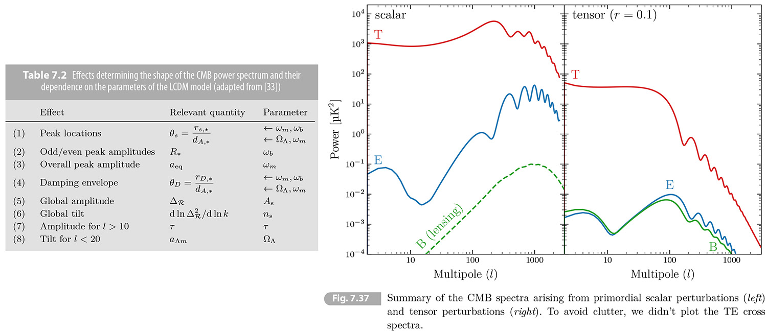
We explained how the shape of the CMB power spectrum depends on the 𝛬CDM parameters {𝛢𝑠, 𝑛𝑠, 𝜔𝑏, 𝜔𝑚, 𝛺𝛬, 𝜏}. The main effects are summarized in Table 7.2. Three length scales are imprinted in the spectrum:
• 𝑟𝑠,*: The peak location depend on the sound horizon at last-scattering.
• 𝑘𝐷-1: The damping of the spectrum is determined by the diffusion scale.
• 𝑑𝛢,*: The map to angular scales depends on the distance to last-scattering.
The sound horizon and the diffusion scale are fixed by pre-combination physics ad hence in the 𝛬CDM model depend only on 𝜔𝑏 and 𝜔𝑚 (for fixed radiation density). These parameters also determine the peak heights through baryon loading (𝜔𝑏) and radiation driving (𝜔𝑚). The angular diameter distance to last-scattering is sensitive to the geometry (𝛺𝛬, 𝐻0) and the energy content (𝛺𝑚, 𝛺𝛬) of the late universe.
Finally, a brief introduction to CMB polarization was given. It was shown that polarization is generated by scattering if the temperature anisotropies seen by the electrons have a quadrupole moment. The signal can be seperated into a curl-free E-mode and a divergenceless B-mode. We prove that density fluctuations only produce E-modes, making the B-mode signal a unique signature of primordial gravitational waves (see Fig. 7.37). As we will discuss in the next chapter, these gravitational waves carry critical information about the physics of inflation.
Selected Problems
7.1 CMB dipole
The CMB is assumed to be isotropic with temperature 𝛵 in an inertial frame 𝑆. Consider another inertial frame 𝑆', moving with velocity 𝑣 with respect to 𝑆. The energy 𝐸 and 3-momentum 𝐩 of a particle in the two frames are related by a Lorentz transformation
(7.1) 𝐸 = 𝛾(𝐸' + 𝐯 ⋅ 𝐩'),
where 𝛾 = 1/√(1 - 𝑣2/𝑐2). A photon has 𝐸 = 𝑝𝑐.
1. Show that the CMB will also appear thermal in 𝑆', but with an anisotropic temperature
(7.1.1) 𝛵'(𝜃') = 𝛵/𝛾[1 - 𝑣/𝑐 cos(𝜃')] = 𝛵[1 + 𝑣/𝑐 cos(𝜃') + 𝑂(𝑣2/𝑐2)],
where 𝜃' is the angle between the velocity 𝐯 and the direction of incoming photon 𝐧̂ = -𝐩̂.
[Solution] First, we know that 𝐧̂ ⋅ 𝐯 = cos(𝜃') = -𝐩̂' ⋅ 𝐯, we can start
(a) 𝐸 = 𝛾(𝐸' + 𝐯 ⋅ 𝐩') = 𝛾[𝐸' - 𝑝'𝑐 𝑣/𝑐 cos(𝜃')] = 𝛾𝐸'[1 - 𝑣/𝑐 cos(𝜃')], 𝐸'/𝐸 = 1/𝛾[1 - 𝑣/𝑐 cos(𝜃')].
From (3.4) the distribution function for bosons with momentum and no chemical potential, 𝑓(𝐸) = 1/(𝑒𝐸/𝛵 - 1). If 𝐸/𝛵 = 𝐸'/𝛵', it will remain thermal. So we get the equation and then apply Taylor expansion for 𝑣 ≪ 𝑐
(b) 𝛵'(𝜃') = 𝐸'/𝐸 𝛵 = 𝛵/𝛾[1 - 𝑣/𝑐 cos(𝜃')] = 𝛵[1 + 𝑣/𝑐 cos(𝜃') + 𝑂(𝑣2/𝑐2)]. ▮
2. Let 𝛵'+ and 𝛵'- be the maximum and minimum temperatures seen in the frame 𝑆'. Show that
(7.1.2) 𝛵 = √(𝛵'+𝛵'-).
The observed CMB has 𝛵'+ - 𝛵'- ≈ 6.5 mK and 𝛵 = √(𝛵'+𝛵'-) ≈ 2.7 K. How fast we traveling with respect to the universe's preferred inertial frame?
[Solution] Since -1 ≤ cos(𝜃') ≤ 1 we have
(a) 𝛵'+ = 𝛵/𝛾(1 - 𝑣/𝑐), 𝛵'- = 𝛵/𝛾(1 + 𝑣/𝑐).
(b) 𝛵'+𝛵'- = 𝛵2/𝛾2[1 - (𝑣/𝑐)2] ≈ 𝛵2, hence
(c) 𝛵 = √(𝛵'+𝛵'-).
From (7.1.1) we get
(d) 𝛵'+ - 𝛵'- ≈ 𝛵(1 + 𝑣/𝑐) - 𝛵(1 - 𝑣/𝑐) = 2𝛵 𝑣/𝑐. hence
(e) 𝑣 = (𝛵'+ - 𝛵'-)/2𝛵 𝑐 = 0.0065 K/5.4 K 𝑐 = 0.0012 𝑐, so we get 𝑣 ≈ 360 km/s. ▮
3. Consider now the cosmic neutrino background (C𝜈B). The neutrinos have a small mass and so 𝐸2 = 𝑝2𝑐2 + 𝑚2𝑐4. Today, the neutrinos are traveling at non-relativistic speeds. Show that the C𝜈B will not be thermal, even at a fixed angle.
[Solution] If C𝜈B is thermal, it must be that 𝐸/𝛵 = 𝐸'/𝛵'. But from [P7.1.1 (a-b)] we have
(a) 𝐸 = 𝛾[𝐸' - 𝑝'𝑐 𝑣/𝑐 cos(𝜃')], 𝑝'𝑐/𝐸' = √[1 - (𝑚𝑐2/𝐸')2]
(b) 𝐸' = √( 𝑝'2𝑐2 + 𝑚2𝑐4),
(c) 𝐸/𝛵 = 𝛾𝐸'/𝛵 (1 - √[1 - (𝑚𝑐2/𝐸')2] 𝑣/𝑐 cos(𝜃'))
which cannot be written as 𝐸'/𝛵'. Therefore C𝜈B today does not have a thermal spectrum. ▮
7.2 Sound horizon
Show that the sound horizon can be written as
(7.2) 𝑟𝑠(𝜂) = 2/3𝑘eq √(6/𝑅eq) ln [√{1 + 𝑅(𝜂)} + √{𝑅(𝜂) + 𝑅eq}]/(1 + √𝑅eq),
where 𝑘eq = 𝓗(𝜂eq) and 𝑅eq = 𝑅(𝜂eq). Determine the size of the horizon at last-scattering, using the best-fit values of the cosmological parameters. What CMB multipole moment does this scale corresponds to?
[Solution] From (6.198) and (6.200) the sound horizon is
(a) 𝑟𝑠(𝜂) ≡ ∫𝜂0 𝑐𝑠(𝜂') d𝜂' = ∫𝜂0 d𝜂'/√3[1 + 𝑅(𝜂')]
From (2.162-3) we have
(b) 𝑎(𝜂) = 𝑎eq[(𝜂/𝜂*)2 + 2(𝜂/𝜂*)], 𝜂* = 𝜂eq/(√2 - 1)
(c) 𝓗 ≡ 𝑎ʹ/𝑎 = [2(𝜂/𝜂*) + 2]/𝜂*[(𝜂/𝜂*)2 + 2(𝜂/𝜂*)],
(d) 𝑘eq = 𝓗(𝜂eq) = 2√2/𝜂*
(e) 𝑅 ≡ 3/4 𝜌̄𝑏/𝜌̄𝛾 = 0.6 (𝛺𝑏𝘩2/0.02)(𝑎/10-3) = 0.6 (𝛺𝑏𝘩2/0.02) 1000/(1 + 𝑧) [RE (6.191)]
(f) 𝑅(𝜂) = 𝑅eq[(𝜂/𝜂*)2 + 2(𝜂/𝜂*)].
(g) 𝑟𝑠(𝜂) = ∫𝜂0 d𝜂'/√3[1 + 𝑅eq{(𝜂'/𝜂*)2 + 2(𝜂'/𝜂*)}]
(h) 𝑟𝑠(𝜂) = 2/3𝑘eq √(6/𝑅eq) ln [√{1 + 𝑅(𝜂)} + √{𝑅(𝜂) + 𝑅eq}]/(1 + √𝑅eq)
From Table 2.1 and Table 3.3 we can find the sound horizon at last-scattering, we find
(i) 𝑅* = 𝑅(𝑧* = 1090) ≈ 0.6 and 𝑅eq = 𝑅(𝑧eq = 3400) ≈ 0.2.
From Appendix (C.22) the measured value of the equality scale is 𝑘eq ≈ 0.01, so we get
(j) 𝑟𝑠(𝜂*) = 1.45/𝑘eq ≈ 145 Mpc
From (7.54) with 𝑘𝑟𝑠,* > 1, 𝑙 ~ 𝑘𝜒* and 𝜒* ≈ 14 Gpc, so we find the multipole moment is
(k) 𝑙𝑠 > 𝜒*/𝑟𝑠,* ≈ 100. ▮
7.4 WKB solution
Consider the equation of a damped harmonic oscillator
(7.4) 𝑢ʺ + 𝛾(𝜂)𝑢ʹ + 𝜔2(𝜂)𝑢 = 0,
where 𝛾 > 0. We assume that the frequency is slowly varing, in the sense that 𝜔ʹ ≪ 𝜔2.
1. Let 𝑢 ≡ 𝑓𝑣 and find the function 𝑓(𝜂) that removes the damping term. Show that the oscillator ewquation becomes
(7.4.1) 𝑣ʺ + [𝜔2 -1/2 (𝛾ʹ + 𝛾2)] 𝑣 = 0,
which reduces to 𝑣ʺ + 𝜔2𝑣 = 0 for 𝜔2 ≫ {𝛾ʹ, 𝛾2}.
[Solution] Substituting 𝑢 ≡ 𝑓𝑣 into (P7.4), we obtain
(a) (𝑓𝑣)ʺ + 𝛾(𝑓𝑣)ʹ + 𝜔2(𝑓𝑣) = 0 ⇒ 𝑣ʺ + (2𝑓ʹ/𝑓 + 𝛾)𝑣ʹ + (𝑓ʺ/𝑓 + 𝛾𝑓ʹ/𝑓 + 𝜔2)𝑣 = 0.
We can remove the damping term as
(b) 2𝑓ʹ/𝑓 + 𝛾 = 0 ⇒ 𝑓 = exp[-1/2 ∫𝜂 𝛾(𝜂') d𝜂'].
Substituting 𝑓 into (a), we get
(c) 𝑣ʺ + [𝜔2 -1/2 (𝛾ʹ + 𝛾2)] 𝑣 = 0.
For 𝜔2 ≫ {𝛾ʹ, 𝛾2} we find
(d) 𝑣ʺ + 𝜔2𝑣 = 0. ▮
2. Consider the ansatz 𝑣 = 𝑒𝑖𝛿, with ∣𝛿ʺ∣ ≪ (𝛿ʹ)2. Show that the solution of the oscillator equation is
(7.4.2) 𝑣 ∝ 𝜔-1/2exp(±𝑖 ∫𝜂 𝜔 d𝜂').
[Solution] Substituting the ansatz into (P7.4.1 d) gives
(a) 𝑖𝛿ʺ - (𝛿ʹ)2 + 𝜔2 = 0
Since ∣𝛿ʺ∣ ≪ (𝛿ʹ)2, we have
(b) - (𝛿ʹ)2 + 𝜔2 = 0 ⇒ 𝛿 = ± ∫𝜂 𝜔 d𝜂' ⇒ 𝛿ʺ = ±𝜔ʹ
Substituting 𝛿ʺ = ±𝜔ʹ into (a) we find
(c) 𝛿ʹ = ±𝜔(1 ± 𝑖𝜔ʹ/𝜔2)1/2 ≈ ±𝜔 + 𝑖𝜔ʹ/2𝜔 ⇒ 𝛿 = ± ∫ + 𝜂 𝜔 d𝜂' + 𝑖ln 𝜔1/2, hence
(d) 𝑣 = 𝑒𝑖𝛿 ∝ 𝜔-1/2exp(±𝑖 ∫𝜂 𝜔 d𝜂'). ▮
3. Apply these results to the equation
(P7.4.3) 𝛿𝛾ʺ + 𝑅ʹ/(1+ 𝑅) 𝛿𝛾ʹ + 𝑘2/3(1 + 𝑅) 𝛿𝛾 = 0.
Show that the amplitude of the oscillations scales as 𝛿𝛾 ∝ (1 + 𝑅)-1/4.
[Solution] Comparing (P7.4.3) with equation (P7.4) we can set
(a) 𝛾 = 𝑅ʹ/(1+ 𝑅) = d/d𝜂 ln(1 + 𝑅), 𝜔 = 𝑘/√3(1 + 𝑅) = 𝑘𝑐s ∝(1 + 𝑅)-1/2 .
(b) 𝑓 = exp[-1/2 ∫𝜂 𝛾(𝜂') d𝜂'] = (1+ 𝑅)-1/2.
(c) 𝑣 ∝ 𝜔-1/2exp(±𝑖 ∫𝜂 𝜔 d𝜂') ∝(1 + 𝑅)1/4 𝑒±𝑖𝑘𝑐s, hence
(d) 𝛿𝛾 = 𝑓𝑣 = (1+ 𝑅)-1/2𝑣 ∝(1+ 𝑅)-1/4. ▮
7.6 Temperature anisotropies from tensor modes
Derive the temperature anisotropies induced by primordial tensor modes, i.e. metric perturbations of the form
(7.6) d𝑠2 = 𝑎2(𝜂) [-𝑑𝜂2 + (𝛿𝑖𝑗 + 𝘩𝑖𝑗)d𝑥𝑖d𝑥𝑗],
where 𝘩𝑖𝑗 is transverse and traceless.
1. By considering the geodesic equation in the presence of the tensor perturbations, show that the energy of a photon evolves as
(7.6.1) d ln(𝑎𝐸)/d𝜂 = -1/2 𝘩𝑖𝑗ʹ 𝑝̂𝑖 𝑝̂𝑗,
where 𝑝̂𝑖 is a unit vector in the photon's direction of propagation.
Hints: To linear order in 𝘩𝑖𝑗, the relevant connection coefficients are 𝛤000 = 𝓗 and 𝛤0𝑖𝑗 = 𝓗𝛿𝑖𝑗 + 𝓗𝘩𝑖𝑗 + 1/2 𝘩𝑖𝑗ʹ.
[Solution] From the geodesic equation
(a) d𝑃𝜇/d𝜆 = -𝛤𝜇𝜈𝜌𝑃𝜈𝑃𝜌, where 𝑃𝜇 = d𝑥𝜇/d𝜆.
(b) d𝑃𝜇/d𝜆 = d𝜂/d𝜆 d𝑃𝜇/d𝜂 = 𝑃0 d𝑃𝜇/d𝜂 = 𝐸/𝑎 d𝑃𝜇/d𝜂
We can find the time-component of the geodesic equation as
(c) 𝐸/𝑎 d𝑃0/d𝜂 = 𝐸/𝑎 d(𝐸/𝑎)/d𝜂 = -𝐸2/𝑎3 d𝑎/d𝜂 = -𝐸2/𝑎2 d ln(𝑎𝐸)/d𝜂 = -𝛤0𝜈𝜌𝑃𝜈𝑃𝜌 = -𝐸2/𝑎2 [𝛤000 - 𝛤0𝑖𝑗(𝑝̂𝑖 - 𝘩𝑖𝑘 𝑝̂𝑘)(𝑝̂𝑗 - 𝘩𝑗𝑙 𝑝̂𝑙)] ,
where 𝑃𝑖/𝑃0 = 𝑝̂𝑖 - 𝘩𝑖𝑘 𝑝̂𝑘.
Substituting the equations in the above hints, we get
(d) d ln(𝑎𝐸)/d𝜂 = 𝓗 - (𝓗𝛿𝑖𝑗 + 𝓗𝘩𝑖𝑗 + 1/2 𝘩𝑖𝑗ʹ)(𝑝̂𝑖 - 𝘩𝑖𝑘 𝑝̂𝑘)(𝑝̂𝑗 - 𝘩𝑗𝑙 𝑝̂𝑙).
We may drop all terms which are beyond linear order in 𝘩𝑖𝑗, then we obtain
(e) d ln(𝑎𝐸)/d𝜂 = -1/2 𝘩𝑖𝑗ʹ 𝑝̂𝑖 𝑝̂𝑗. ▮
2. Assuming instanteneous decoupling, show that the line-of-sight solution for the induced temperature anisotropy is
(7.6.2) 𝛩(𝑡)(𝐧̂) = -1/2 ∫𝜂0𝜂* d𝜂 ∫ d3𝑘/(2π)3 𝘩𝑖𝑗ʹ(𝜂, 𝐤) 𝑛̂𝑖 𝑛̂𝑗 𝑒𝑖𝑘𝜒(𝜂) 𝐤̂⋅𝐧̂,
where 𝜒(𝜂) = 𝜂0 - 𝜂 in a flat universe.
[Solution] Tensor induced contributtion to the temperature anisotropies comes from the free-streaming effect:
(a) d𝛩(𝑡)/d𝜂 = d ln(𝑎𝐸)/d𝜂 = -1/2 𝘩𝑖𝑗ʹ 𝑝̂𝑖 𝑝̂𝑗.`
(b) 𝛩(𝑡)(𝐧̂) = -1/2 ∫𝜂0𝜂* d𝜂 𝘩𝑖𝑗ʹ(𝜂, 𝐱(𝜂)) 𝑛̂𝑖 𝑛̂𝑗,
where 𝐱(𝜂) ≡ 𝜒(𝜂)𝐧̂. If we write 𝘩𝑖𝑗ʹ in terms of its Fourier transform, we get
(c) 𝛩(𝑡)(𝐧̂) = -1/2 ∫𝜂0𝜂* d𝜂 ∫ d3𝑘/(2π)3 𝘩𝑖𝑗ʹ(𝜂, 𝐤) 𝑛̂𝑖 𝑛̂𝑗 𝑒𝑖𝑘𝜒(𝜂) 𝐤̂⋅𝐧̂. ▮
3. Consider a sigle gravitational wave with wavevector 𝐤 pointing 𝑧-direction and write 𝘩𝑖𝑗 in terms of its two polarization modes,
⌈ 𝘩+ 𝘩× 0 ⌉ ⌈ 𝘩+ 𝘩× 0 ⌉
(7.6.3a) 𝘩𝑖𝑗 = ┃𝘩× -𝘩+ 0┃ * ipad view ┃𝘩× -𝘩+ 0┃ * PC view
⌊ 0 0 0 ⌋ ⌊ 0 0 0 ⌋
Show that
(7.6.3b) 𝘩𝑖𝑗ʹ 𝑛̂𝑖 𝑛̂𝑗 = sin2(𝜃)[𝘩+ʹ cos(2𝜙) + 𝘩×ʹ cos(2𝜙)],
where 𝜃 and 𝜙 are the angles of 𝐧̂ in polar coordinates.
[Solution] The coordinates of the line-of-sight direction of the incoming photons are
(a) 𝐧̂ = [sin(𝜃)cos(𝜙), sin(𝜃)sin(𝜙), cos(𝜃)].
(b) 𝘩𝑖𝑗ʹ 𝑛̂𝑖 𝑛̂𝑗 = 𝘩+ʹ[(𝑛̂𝑥)2 - (𝑛̂𝑦)2] + 2𝘩×ʹ𝑛̂𝑥𝑛̂𝑦 = sin2(𝜃)[𝘩+ʹ cos(2𝜙) + 𝘩×ʹ cos(2𝜙)]. ▮
4. It is convenient to transform to the helicity basis, where 𝘩±2 ≡ 𝘩+ ∓ 𝑖𝘩× (see Section 6.5). Show that the integrand in (P7.6.2) then becomes
(7.6.4) 𝓘(𝜂, 𝑘𝐳̂) = -√2π/15 ∑𝜆=±2 𝘩𝜆ʹ(𝜂, 𝑘𝐳̂) 𝑌2,𝜆(𝐧̂) 𝑒𝑖𝑘𝜒cos(𝜃),
where cos(𝜃) ≡ 𝐳̂ ⋅ 𝐧̂.
[Solution] Since 𝘩±2 ≡ 𝘩+ ∓ 𝑖𝘩×, we obtain
(a) 𝘩+ = 1/2 (𝘩+2 + 𝘩-2), 𝘩× = 1/2 (𝘩+2 - 𝘩-2)
substituting this into (P7.6.3.2) and reffering to equations (D.6) in Appendix D.2 we get
(b) 𝘩𝑖𝑗ʹ 𝑛̂𝑖 𝑛̂𝑗 = sin2(𝜃)[𝘩+ʹ cos(2𝜙) + 𝘩×ʹ cos(2𝜙)] = sin2(𝜃) (𝘩+2ʹ [cos(2𝜙) + 𝑖 sin(2𝜙)]/2 + 𝘩-2ʹ [cos(2𝜙) + 𝑖 sin(2𝜙)]/2)
= 1/2 sin2(𝜃) (𝘩+2ʹ 𝑒2𝑖𝜙 + 𝘩-2ʹ 𝑒-2𝑖𝜙) = -√8π/15 [𝘩+2ʹ 𝑌2,+2(𝐧̂) + 𝘩-2ʹ 𝑌2,-2(𝐧̂)].
Then (P7.6.2) becomes [verification needed]
(c) 𝓘(𝜂, 𝑘𝐳̂) = -√2π/15 ∑𝜆=±2 𝘩𝜆ʹ(𝜂, 𝑘𝐳̂) 𝑌2,𝜆(𝐧̂) 𝑒𝑖𝑘𝜒cos(𝜃), ▮
|
|
|